Awesome
CAI NEURAL API 

<img align="right" src="docs/cai.png" height="192">
CAI NEURAL API is a pascal based deep learning neural network API optimized for AVX, AVX2 and AVX512 instruction sets plus
OpenCL capable devices including AMD, Intel and NVIDIA. This API has been tested under Windows and Linux.
This project is a subproject from a bigger and older project called CAI and is sister to Keras based K-CAI NEURAL API. You can find trained neural network models in the pre-trained-neural-api-networks repository.
Intro Videos
 |  |  |
|---|---|---|
| Basics of Neural Networks in Pascal - Loading and Saving | Neural Networks for Absolute Beginners! Learning a Simple Function | Coding a Neural Network in Pascal that Learns to Calculate the Hypotenuse |
Why Pascal?
- The Pascal computer language is easy to learn. Pascal allows developers to make a readable and understandable source code.
- You'll be able to make super-fast native code and at the same time have a readable code.
- This API can outperform some major APIs in some architectures.
Prerequisites
You'll need Lazarus development environment. If you have an OpenCL capable device, you'll need its OpenCL drivers. Many examples use the CIFAR-10 dataset. You'll also find examples for the CIFAR-100, MNIST, Fashion MNIST and the Places365-Standard Small images 256x256 dataset.
Will It Work with Delphi?
This project is Lazarus based. That said, as of release v2.0.0, a number of units do compile with Delphi and you can create and run neural networks with Delphi. You'll be able to compile these units with Delphi: neuralvolume, neuralnetwork, neuralab, neuralabfun, neuralbit, neuralbyteprediction, neuralcache, neuraldatasets, neuralgeneric, neuralplanbuilder, Neural OpenCL, Neural Threading and neuralfit.
Installation
Clone this project, add the neural folder to your Lazarus unit search path and you'll be ready to go!
A.I. Powered Support
You can get A.I. powered help from these tools:
- CAI Neural API support at Poe (free).
- CAI Neural API support at Poe.
- CAI Neural API support at ChatGPT4.
Documentation
In this readme file, you’ll find information about:
- Easy examples.
- Simple image classification examples.
- Youtube videos.
- Advanced examples.
- Data structures (Volumes).
- Neural network layers.
- Dataset support.
- Training (fitting) your neural network.
- Parallel computing.
- Other scientific publications from the same author.
Easy Examples First Please!
You can click on the image above to watch the video.
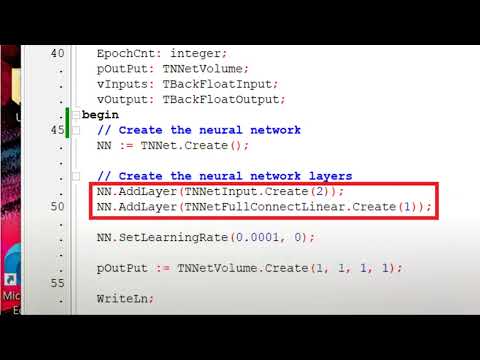
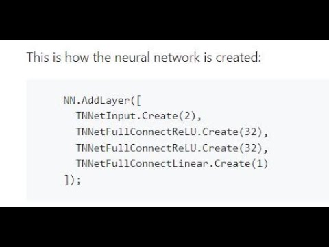
Assuming that you would like to train a neural network to learn a function that has 2 inputs and one output, you could start with something like this:
    NN.AddLayer([
      TNNetInput.Create(2),
      TNNetFullConnectReLU.Create(32),
      TNNetFullConnectReLU.Create(32),
      TNNetFullConnectLinear.Create(1)
    ]);
The example above has 2 inputs (TNNetInput), 2 dense layers (TNNetFullConnectReLU) with 32 neurons each and one output (TNNetFullConnectLinear).
You can learn more about how to build and train simple neural networks at the following source code examples:
- Only one neuron.
- Training a neural network to learn the hypotenuse function
- Training a neural network to learn the hypotenuse function with FitLoading
- Training a neural network to learn boolean functions AND, OR and XOR with neuralfit unit
- Training a neural network to learn boolean functions AND, OR and XOR without neuralfit unit
Loading and Saving Neural Networks
Loading is very easy:
    NN := TNNet.Create;
    NN.LoadFromFile('MyTrainedNeuralNetwork.nn');
Saving is as easy:
NN.SaveToFile('MyTrainedNeuralNetwork.nn');
Simple Image Classification Examples
CIFAR-10 Image Classification Example
The CIFAR-10 dataset is a well-known collection of images commonly used to train machine learning and computer vision algorithms. It was created by the Canadian Institute for Advanced Research (CIFAR). It contains 60K 32x32 color images. The images are classified into 10 different classes, with 6,000 images per class. The classes represent airplanes, cars, birds, cats, deer, dogs, frogs, horses, ships, and trucks. Despite its relatively low resolution and small size, CIFAR-10 can be challenging for models to achieve high accuracy, making it a good dataset for testing advancements in machine learning techniques.
Follows a source code example for the CIFAR-10 image classification:
NN := TNNet.Create();
NN.AddLayer([
  TNNetInput.Create(32, 32, 3), //32x32x3 Input Image
  TNNetConvolutionReLU.Create({Features=}16, {FeatureSize=}5, {Padding=}0, {Stride=}1, {SuppressBias=}0),
  TNNetMaxPool.Create({Size=}2),
  TNNetConvolutionReLU.Create({Features=}32, {FeatureSize=}5, {Padding=}0, {Stride=}1, {SuppressBias=}0),
  TNNetMaxPool.Create({Size=}2),
  TNNetConvolutionReLU.Create({Features=}32, {FeatureSize=}5, {Padding=}0, {Stride=}1, {SuppressBias=}0),
  TNNetFullConnectReLU.Create({Neurons=}32),
  TNNetFullConnectLinear.Create(NumClasses),
  TNNetSoftMax.Create()
]);

CreateCifar10Volumes(ImgTrainingVolumes, ImgValidationVolumes, ImgTestVolumes);

WriteLn('Neural Network will minimize error with:');
WriteLn(' Layers: ', NN.CountLayers());
WriteLn(' Neurons:', NN.CountNeurons());
WriteLn(' Weights:', NN.CountWeights());

NeuralFit := TNeuralImageFit.Create;
NeuralFit.InitialLearningRate := fLearningRate;
NeuralFit.Inertia := fInertia;
NeuralFit.Fit(NN, ImgTrainingVolumes, ImgValidationVolumes, ImgTestVolumes, NumClasses, {batchsize}128, {epochs}100);
These examples train a neural network to classify images in classes such as: image has a cat, image has a dog, image has an airplane...
- Simple CIFAR-10 Image Classifier

- Simple CIFAR-10 Image Classifier with OpenCL
- Many neural network architectures for CIFAR-10 image classification
- MNIST, Fashion MNIST and CIFAR-100
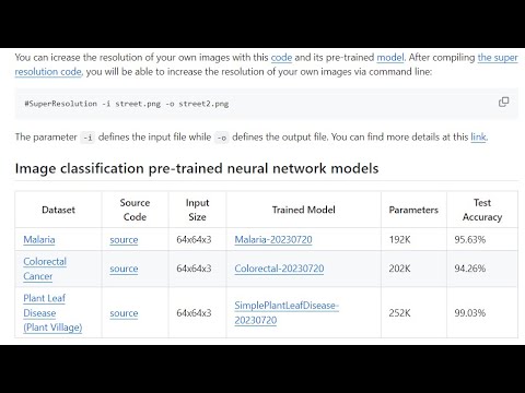
You can save and load trained models (neural networks) with TNNet.SaveToFile and TNNet.LoadFromFile. The file format is portable meaning that you can train on CPU and run on GPU or train in AMD and run on ARM as examples. The following code shows a simple example for image classification loading a pre-trained model:
  procedure ClassifyOneImageSimple;
  var
    NN: TNNet;
    ImageFileName: string;
    NeuralFit: TNeuralImageFit;
  begin
    WriteLn('Loading Neural Network...');
    NN := TNNet.Create;
    NN.LoadFromFile('SimplePlantLeafDisease-20230720.nn');
    NeuralFit := TNeuralImageFit.Create;
    ImageFileName := 'plant/Apple___Black_rot/image (1).JPG';
    WriteLn('Processing image: ', ImageFileName);
    WriteLn(
      'The class of the image is: ',
      NeuralFit.ClassifyImageFromFile(NN, ImageFileName)
    );
    NeuralFit.Free;
    NN.Free;
  end;
Youtube Videos
| | |
|---|---|---|
| Basics of Neural Networks in Pascal - Loading and Saving | Neural Networks for Absolute Beginners! Learning a Simple Function | Coding a Neural Network in Pascal that Learns to Calculate the Hypotenuse |
 |  |  |
| Pre-trained Neural Networks & Transfer Learning with Pascal's CAI Neural API | Coding a Neural Network in Pascal that Learns the OR Boolean Operation | A Dive into Identity Shortcut Connection - The ResNet building block |
 |  |  |
| Increasing Image Resolution with Neural Networks | Ultra Fast Single Precision Floating Point Computing | AVX and AVX2 Code Optimization |
Some videos make referrence to uvolume unit. The current neuralvolume unit used to be called uvolume. This is why it's mentioned.
Advanced Examples
Although these examples require deeper understanding about neural networks, they are very interesting:
- Identity Shortcut Connection - ResNet building block
- ResNet-20 - includes a web server example
- DenseNetBC L40
- Separable Convolutions - MobileNet building block
- Gradient Ascent - Visualizing patterns from inner neurons in image classification <p><img src="https://github.com/joaopauloschuler/neural-api/blob/master/docs/gradientascent3layer.jpg" height="130"></img></p>
- Artificial Art - Let a neural network produce art via a generative adversarial network <p><img src="https://github.com/joaopauloschuler/neural-api/blob/master/docs/art1.png" height="130"></img></p>
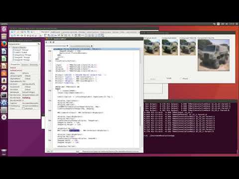
- Super Resolution - A neural network learns how to increase image resolution<p><img src="examples/SuperResolution/results/building_result.png"></img></p>
- CIFAR-10 Resized - A program that resizes CIFAR-10 and CIFAR-100 images to 64x64 and 128x128 pixels.<p><img src="https://github.com/joaopauloschuler/neural-api/blob/master/examples/SuperResolution/results/bird.png?raw=true"> </img></p><p><img src="https://github.com/joaopauloschuler/neural-api/blob/master/examples/SuperResolution/results/stealth.png?raw=true"> </img></p>
- Autoencoder - Shows an autoencoder built with hyperbolic tangents and trained with Tiny ImageNet 200. <p><img src="docs/autoencoder_small.png"></img></p>
There are also some older code examples that you can look at.
Volumes
Volumes behave like dynamically created arrays. They are the main array like structure used by this API. TNNetVolume class allows you to create volumes that can be accessed as 1D, 2D or 3D arrays and be operated with Advanced Vector Extensions (AVX) - Single Instruction Multiple Data (SIMD) instruction set. The usual way to create a volume is:
constructor Create(pSizeX, pSizeY, pDepth: integer; c: T = 0);
You can access the data as 1D or 3D with:
property Raw[x: integer]: T read GetRaw write SetRaw;
property Data[x, y, d: integer]: T read Get write Store; default;
Your code will look like this:
// Usage Examples
vInput := TNNetVolume.Create(32, 32, 3);
vInput[1, 1, 1] := 1;
vInput[2, 2, 2] := vInput[1, 1, 1] + 1;
vInput.Raw[10] := 5;

vInput.RandomizeGaussian();
WriteLn('Avg: ', vInput.GetAvg());
WriteLn('Variance: ', vInput.GetVariance());
WriteLn('Std Dev: ', vInput.GetStdDeviation());

WriteLn('Multiplying by 10');
vInput.Mul(10);
WriteLn('Avg: ', vInput.GetAvg());
WriteLn('Variance: ', vInput.GetVariance());
WriteLn('Std Dev: ', vInput.GetStdDeviation());
As examples, you can add, subtract, multiply and calculate dot products with:
procedure Add(Original: TNNetVolume); overload;
procedure Sub(Original: TNNetVolume); overload;
procedure Mul(Value: Single); overload;
function DotProduct(Original: TNNetVolume): TNeuralFloat; overload;
In the case that you need the raw position or raw pointer to an element of the volume, you can get with:
function GetRawPos(x, y, d: integer): integer; overload;
function GetRawPos(x, y: integer): integer; overload;
function GetRawPtr(x, y, d: integer): pointer; overload;
function GetRawPtr(x, y: integer): pointer; overload;
function GetRawPtr(x: integer): pointer; overload;
You can easily operate volumes with OpenCL via TEasyOpenCLV:
  TEasyOpenCLV = class (TEasyOpenCL)
    public
      function CreateBuffer(flags: cl_mem_flags; V: TNNetVolume): cl_mem; overload;
      function CreateInputBuffer(V: TNNetVolume): cl_mem; overload;
      function CreateHostInputBuffer(V: TNNetVolume): cl_mem; overload;
      function CreateOutputBuffer(V: TNNetVolume): cl_mem; overload;
      function CreateBuffer(V: TNNetVolume): cl_mem;  overload;

      function WriteBuffer(buffer: cl_mem; V: TNNetVolume; blocking: cl_bool = CL_FALSE): integer;
      function ReadBuffer(buffer: cl_mem; V: TNNetVolume; blocking: cl_bool = CL_TRUE): integer;

      function CreateAndWriteBuffer(V: TNNetVolume; var buffer: cl_mem): integer; overload;
      function CreateAndWriteBuffer(V: TNNetVolume): cl_mem; overload;
      function CreateWriteSetArgument(V: TNNetVolume; kernel:cl_kernel; arg_index: cl_uint): cl_mem;
      function CreateOutputSetArgument(V: TNNetVolume; kernel:cl_kernel; arg_index: cl_uint): cl_mem;
  end;
Volume Pairs, Volume Lists and Volume Pair Lists
Volumes can be organized in pairs:
  /// Implements a pair of volumes
  TNNetVolumePair = class(TObject)
    protected
      FA: TNNetVolume;
      FB: TNNetVolume;
    public
      constructor Create(); overload;
      constructor Create(pA, pB: TNNetVolume); overload;
      constructor CreateCopying(pA, pB: TNNetVolume); overload;

      destructor Destroy(); override;

      property A:TNNetVolume read FA;
      property B:TNNetVolume read FB;
      property I:TNNetVolume read FA;
      property O:TNNetVolume read FB;
  end;
Depending on the problem that you are trying to solve, modelling the training with pairs or pair lists might be helpful. Typically, a pair will be (input, desired output). This is how volume lists and volume pair lists have been implemented:
TNNetVolumeList = class (specialize TFPGObjectList<TNNetVolume>
TNNetVolumePairList = class (specialize TFPGObjectList<TNNetVolumePair>)
Neural Network Layers
The layered structure of artificial neural networks is inspired by the organization of the human brain and nervous system. In the human brain, information processing occurs in a hierarchical manner. Sensory inputs are first processed by lower-level neurons, which extract simple features. These features are then passed on to deeper neurons that combine them to recognize more complex patterns. This hierarchical processing is mirrored in artificial neural networks through the use of stacked layers.
Biological neurons are connected to each other through synapses, forming complex networks. Similarly, in artificial neural networks, neurons in one layer are connected to neurons in the next layer, mimicking this interconnected structure. Biological neurons fire (activate) based on a non-linear response to their inputs. This non-linearity is crucial for the brain's ability to learn complex patterns. In artificial neural networks, we use non-linear activation functions (such as ReLU) to introduce this non-linearity. Different regions of the brain specialize in processing different types of information. For instance, the visual cortex has layers specialized for detecting edges, shapes, and complex objects. This specialization is reflected in artificial neural networks, where different layers can learn to recognize different levels of abstraction.
In the context of artificial neural networks, we can see this biologically-inspired layered approach implemented. For example:
NN := TNNet.Create();
NN.AddLayer([
  TNNetInput.Create(32, 32, 3),
  TNNetConvolutionLinear.Create({neurons=}16, {featuresize}3, {padding}1, {stride}1),
  TNNetReLU6.Create()
]);
This code snippet demonstrates the creation of a neural network with an input layer and a convolutional layer followed by a ReLU6 activation. This structure is inspired by the visual cortex in the brain, where neurons respond to specific patterns in their receptive fields, similar to how convolutional layers operate. The CAI Neural API also supports the creation of more complex, biologically-inspired architectures. These architectures are designed with multiple layers of different types, mirroring the complex structure of the brain.
Artificial neural networks with multiple layers and specialized structures are inspired by the hierarchical and specialized nature of biological neural processing. It's important to note that while artificial neural networks are inspired by biological neural networks, they are highly simplified models. The human brain is far more complex, with various types of neurons, complex connectivity patterns, and mechanisms we don't yet fully understand. However, the layered structure in artificial neural networks has proven to be a powerful approach for solving complex problems in machine learning, inspired by the remarkable capabilities of biological neural networks.
Input Layer
The input layer serves as the gateway to the entire network. It's like the sensory organs of our brain, receiving information from the outside world. Without an input layer, the neural network would have no way to receive and interpret the initial data, making it impossible to perform any meaningful computations or learning tasks. The TNNetInput class implements the input layer.
Fully Connected (Dense) Layers
Fully connected layers, also known as dense layers, are a fundamental component of neural networks. In these layers, every neuron is connected to every neuron in the previous layer, allowing for comprehensive information processing across the entire network.
In the context of the CAI Neural API, fully connected layers are represented by various classes derived from TNNetFullConnect. These layers play a crucial role in transforming input data and learning complex patterns.
The computation process in a fully connected layer involves:
- Multiplying input values by the layer's weights.
- Adding bias terms (if not suppressed).
- Applying an activation function (if present).
Key types of fully connected layers include:
TNNetFullConnectLinear: a basic fully connected layer without an activation function. It performs a linear transformation of the input data.TNNetFullConnectReLU: incorporates the Rectified Linear Unit (ReLU) activation function. ReLU introduces non-linearity by outputting the input for positive values and zero for negative values, helping the network learn complex patterns.TNNetFullConnectSigmoid: applies the sigmoid activation function to the layer's output. Sigmoid squashes the output between 0 and 1, useful for binary classification tasks.
Fully connected layers are typically used in neural network architectures as:
- Hidden layers for processing and transforming features.
- Output layers for producing final predictions.
For example, in the provided context, we see a simple neural network structure:
NN := TNNet.Create();
NN.AddLayer([
  TNNetInput.Create(2),       // Input layer with 2 inputs
  TNNetFullConnect.Create(2), // Hidden fully connected layer with 2 neurons
  TNNetFullConnect.Create(1)  // Output fully connected layer with 1 neuron
]);
| Layer Name | Input/Output Dimensions | Activation | Description |
|---|---|---|---|
TNNetFullConnectLinear | 1D, 2D, or 3D | None | Fully connected layer without an activation function (linear). |
TNNetFullConnect | 1D, 2D, or 3D | tanh | Fully connected layer with tanh as the default activation function. |
TNNetFullConnectReLU | 1D, 2D, or 3D | ReLU | Fully connected layer with ReLU activation. |
TNNetFullConnectSigmoid | 1D, 2D, or 3D | Sigmoid | Fully connected layer with Sigmoid activation. |
TNNet.AddGroupedFullConnect | 1D, 2D, or 3D | Optional | Adds a grouped fully connected layer, inspired by TNNet.AddGroupedConvolution. |
Convolutional Layers
Neurons, filters, and kernels are often used as synonyms in the context of neural networks, particularly in convolutional neural networks (CNNs). They are closely related concepts that are used interchangeably. Here's why:
- Neurons: in artificial neural networks, neurons are the basic computational units. They receive input, process it, and produce an output. In the context of CNNs, the term "neuron" is sometimes used to refer to a single element in a feature map.
- Filters: in CNNs, filters (also called convolution kernels) are small matrices of weights that slide over the input data to detect specific features. Each filter produces a feature map in the output layer.
- Kernels: in image processing and CNNs, kernels are small matrices used for various operations like blurring, sharpening, or edge detection. In the context of CNNs, kernels and filters are essentially the same thing.
The reason these terms are often used synonymously is that they all contribute to the feature detection and transformation process in neural networks:
- A single filter/kernel can be thought of as a specialized neuron that detects a specific feature across the entire input.
- The weights in a filter/kernel are analogous to the weights in a traditional neuron.
- The output of applying a filter/kernel to an input region is similar to the activation of a neuron in response to its inputs.
In practice, when implementing CNNs, the terms "filter" and "kernel" are more commonly used than "neuron" when referring to the convolutional layers. However, the underlying concept of a computational unit that processes input and produces output remains the same across these terms.
Convolutional layers are fundamental building blocks in neural networks, particularly in the field of computer vision and image processing. They are designed to automatically and adaptively learn spatial hierarchies of features from input data, such as images.
In the context of the CAI Neural API, convolutional layers are implemented as classes derived from TNNetConvolutionAbstract. This abstract base class provides the core functionality for convolutional operations.
The structure of a convolutional layer typically includes:
- Input: A multi-dimensional array (usually 3D for images: width, height, and channels).
- Kernels (or filters): small matrices of weights that slide over the input.
- Feature maps: the output produced by applying the kernels to the input.
Key parameters of convolutional layers include:
- Number of features (or filters).
- Feature size (kernel size).
- Padding.
- Stride.
The CAI Neural API offers several types of convolutional layers:
TNNetConvolution: the standard convolutional layer.TNNetConvolutionLinear: a convolutional layer without an activation function.TNNetConvolutionReLU: a convolutional layer with a ReLU activation function.
Convolutional layers are crucial in neural networks because they:
- Automatically learn hierarchical features from data.
- Maintain spatial relationships in the input.
- Reduce the number of parameters compared to fully connected layers.
- Enable the network to be translation-invariant.
In practice, convolutional layers are often used in combination with other layer types, such as pooling layers (e.g., TNNetMaxPool) and normalization layers (e.g., TNNetMovingStdNormalization), to create powerful neural network architectures for tasks like image classification, object detection, and segmentation.
Here's a brief example of how to create a convolutional layer using the CAI Neural API:
NN := TNNet.Create();
NN.AddLayer([
  TNNetInput.Create(32, 32, 3),  // Input layer for 32x32 RGB images
  TNNetConvolutionLinear.Create(
    {Features=}64,     // Number of output features
    {FeatureSize=}5,   // 5x5 kernel size
    {Padding=}2,       // Padding of 2 pixels
    {Stride=}1,        // Stride of 1 pixel
    {SuppressBias=}1   // Suppress bias
  ),
  TNNetReLU6.Create()  // Activation function
]);
This example creates a convolutional layer with 64 features, a 5x5 kernel size, padding of 2, and a stride of 1, followed by a ReLU6 activation function.
These are tha available convolutional layers in CAI:
| Layer Name | Input/Output Dimensions | Activation | Description |
|---|---|---|---|
TNNetConvolutionLinear | 1D, 2D, or 3D | None | Linear convolutional layer without activation. Useful for intermediate layers. |
TNNetConvolution | 1D, 2D, or 3D | tanh | Standard convolutional layer. Versatile for feature extraction in tasks like image recognition. |
TNNetConvolutionReLU | 1D, 2D, or 3D | ReLU | Convolutional layer with ReLU activation. Helps mitigate vanishing gradient problem. |
TNNetConvolutionSwish | 1D, 2D, or 3D | Swish | Convolutional layer with Swish activation. Performs better than ReLU in some cases. |
TNNetConvolutionHardSwish | 1D, 2D, or 3D | Hard Swish | Convolutional layer with Hard Swish activation. It is similar to swish but it's faster. |
TNNetConvolutionSharedWeights | 1D, 2D, or 3D | same as linked layer | Convolutional layer that uses the weights from another layer |
TNNetPointwiseConvLinear | 1D, 2D, or 3D | None | Linear 1x1 convolution. Useful for channel mixing without spatial operations. |
TNNetPointwiseConvReLU | 1D, 2D, or 3D | ReLU | 1x1 convolution with ReLU. Efficient for channel-wise dimensionality reduction or expansion. |
TNNetPointwiseConv | 1D, 2D, or 3D | tanh | 1x1 convolution. Useful for autoencoding architectures. |
TNNetDepthwiseConvLinear | 1D, 2D, or 3D | None | Linear depthwise convolution. Useful when additional non-linearity is not required. |
TNNetDepthwiseConv | 1D, 2D, or 3D | tanh | Depthwise convolution with tanh activation. Reduces computational cost by processing each channel separately. |
TNNetDepthwiseConvReLU | 1D, 2D, or 3D | ReLU | Depthwise convolution with ReLU activation. Combines depthwise efficiency with the benefits of ReLU. |
TNNet.AddSeparableConvLinear | 1D, 2D, or 3D | None | Adds a linear separable convolution. Useful for lightweight models with reduced parameter count. |
TNNet.AddSeparableConvReLU | 1D, 2D, or 3D | ReLU | Adds a separable convolution with ReLU. Combines depthwise and pointwise for efficient feature extraction. |
TNNet.AddConvOrSeparableConv | 1D, 2D, or 3D | Optional | Adds standard or separable convolution. Supports optional ReLU and normalization for versatile design. |
TNNet.AddGroupedConvolution | 1D, 2D, or 3D | Optional | Adds a grouped convolution. Allows efficient parallel processing of input channels. |
Grouped pointwise convolutions are an interesting and efficient variant of standard convolutions in neural networks. Grouped pointwise convolutions are a type of convolution operation where the input channels are divided into groups, and each group is processed separately. This is particularly useful for 1x1 convolutions (pointwise) where the spatial dimensions are not affected. The grouped approach can significantly reduce the number of parameters in a neural network as shown in the papers Grouped Pointwise Convolutions Reduce Parameters in Convolutional Neural Networks and An Enhanced Scheme for Reducing the Complexity of Pointwise Convolutions in CNNs for Image Classification Based on Interleaved Grouped Filters without Divisibility Constraints. By reducing parameters, these convolutions can make models more efficient in terms of computation and memory usage. These convolutions can be combined with other techniques like normalization and intergroup connections. This flexibility allows for the creation of more sophisticated network designs. Grouped pointwise convolutions are particularly useful in efficient network designs, such as mobile or edge computing applications where resource constraints are significant. They allow for maintaining model expressivity while reducing computational requirements.
The grouped pointwise convolutional layers are:
| Layer Name | Input/Output Dimensions | Activation | Description |
|---|---|---|---|
TNNetGroupedPointwiseConvLinear | 1D, 2D, or 3D | None | Linear 1x1 grouped convolution. Useful for channel mixing without spatial operations. |
TNNetGroupedPointwiseConvReLU | 1D, 2D, or 3D | ReLU | 1x1 grouped convolution with ReLU. Efficient for channel-wise dimensionality reduction or expansion. |
TNNetGroupedPointwiseConvHardSwish | 1D, 2D, or 3D | Hard Swish | 1x1 grouped convolution wish fast hard swish activation function. |
Locally Connected Layers
A locally connected layer is a type of neural network layer that shares some similarities with convolutional layers but has some distinct characteristics:
- Structure: Locally connected layers, like convolutional layers, operate on local regions of the input. However, unlike convolutional layers, they do not share weights across different positions in the input.
- Weight independence: Each local region in the input has its own set of weights, which are not shared with other regions. This allows the layer to learn position-specific features.
- Flexibility: Locally connected layers offer more flexibility in learning spatial hierarchies compared to fully connected layers, while still maintaining position-specific information unlike convolutional layers.
- Parameters: These layers typically have more parameters than convolutional layers due to the lack of weight sharing, which can lead to increased computational complexity and memory usage.
- Use cases: Locally connected layers can be useful in scenarios where position-specific features are important, such as in face recognition tasks where different parts of the face have distinct characteristics based on their location.
| Layer Name | Input/Output Dimensions | Activation | Description |
|---|---|---|---|
TNNetLocalConnectLinear | 1D, 2D, or 3D | None | Locally connected layer with ReLU activation. |
TNNetLocalConnect | 1D, 2D, or 3D | tanh | Locally connected layer with htan as the default activation function. |
TNNetLocalConnectReLU | 1D, 2D, or 3D | ReLU | Locally connected layer with ReLU activation. |
Min / Max / Avg Pools
Max, min, and avg poolings are downsampling techniques used in neural networks, particularly in convolutional neural networks (CNNs). Let's explore each of these pooling types as implemented in the CAI Neural API:
- Max Pooling (
TNNetMaxPool): Max pooling selects the maximum value from a defined region of the input.
- It reduces spatial dimensions while retaining the most prominent features.
- Useful for detecting specific features regardless of their position in the input.
- Min Pooling (
TNNetMinPool): Min pooling selects the minimum value from a defined region of the input.
- It can be useful for detecting dark features or gaps in the input.
- Less common than max pooling but valuable in specific scenarios.
- Average Pooling (
TNNetAvgPool): Average pooling calculates the average value of a defined region of the input.
- It smooths the input and can help in reducing noise.
- Often used when we want to preserve more contextual information compared to max pooling.
Unique pooling variants in the API:
- TNNetMinMaxPool: Performs both max and min pooling and concatenates the results.
- TNNetAvgMaxPool: Combines average and max pooling.
Backpropagation in pooling layers: During backpropagation, pooling layers distribute the gradient differently:
- Max Pooling: The gradient is passed only to the neuron that had the maximum value during the forward pass.
- Min Pooling: Similar to max pooling, but for the minimum value.
- Average Pooling: The gradient is divided equally among all neurons in the pooling region.
The CAI Neural API implements these backpropagation methods in the respective Backpropagate() functions of each pooling class.
Deconvolution (Upsampling) counterparts: The API also provides deconvolution or upsampling layers, which can be seen as the inverse operations of pooling:
TNNetDeMaxPool: a deconvolution layer that can upsample the input.TNNetUpsample: also known as depth_to_space, this layer can increase the spatial dimensions of the input.
These layers are crucial in architectures like autoencoders or in tasks requiring upsampling, such as image segmentation.
When to use each pooling type:
- Max Pooling: it is useful for detecting features regardless of their exact location. It's commonly used in classification tasks.
- Min Pooling: it is useful when the absence of features is important, or when working with inverted data.
- Average Pooling: it is good for preserving more context and reducing noise. Often used in later layers of the network.
TNNetMinMaxPool: used when you want to capture both the presence and absence of features.TNNetAvgMaxPool: used when you need to balance between preserving prominent features and maintaining context.
| Layer Name | Input/Output Dimensions | Description |
|---|---|---|
TNNetAvgPool | 1D, 2D, or 3D | Average pooling layer for reducing spatial dimensions. |
TNNetMaxPool | 1D, 2D, or 3D | Max pooling layer for reducing spatial dimensions. |
TNNetMinPool | 1D, 2D, or 3D | Min pooling layer for reducing spatial dimensions. |
TNNet.AddMinMaxPool | 1D, 2D, or 3D | Performs both min and max pooling, then concatenates the results. |
TNNet.AddAvgMaxPool | 1D, 2D, or 3D | Performs both average and max pooling, then concatenates the results. |
The CAI Neural API also provides specialized versions:
TNNetMaxChannelandTNNetMinChannel: perform max and min operations across the entire channel into a single number per channel.TNNetAvgChannel: averages the entire channel into a single number per channel.
| Layer Name | Input/Output Dimensions | Description |
|---|---|---|
TNNetAvgChannel | 2D or 3D (output: 1D) | Calculates the average value per channel. |
TNNetMaxChannel | 2D or 3D (output: 1D) | Calculates the maximum value per channel. |
TNNetMinChannel | 2D or 3D (output: 1D) | Calculates the minimum value per channel. |
TNNet.AddMinMaxChannel | 1D, 2D, or 3D | Performs both min and max channel operations, then concatenates the results. |
TNNet.AddAvgMaxChannel | 1D, 2D, or 3D | Performs both average and max channel operations, then concatenates the results. |
Trainable Normalization Layers Allowing Faster Learning/Convergence
Normalization layers may offer:
- Improved training stability.
- Better generalization.
- Potential for faster convergence.
The available normalization techniques are:
- Zero-centering (
TNNetChannelZeroCenter). - Standard deviation normalization (
TNNetMovingStdNormalization,TNNetChannelStdNormalization).
| Layer Name | Input/Output Dimensions | Description |
|---|---|---|
TNNetChannelZeroCenter | 1D, 2D, or 3D | Trainable zero-centering normalization. |
TNNetMovingStdNormalization | 1D, 2D, or 3D | Trainable standard deviation normalization. |
TNNetChannelStdNormalization | 1D, 2D, or 3D | Trainable per-channel standard deviation normalization. |
TNNet.AddMovingNorm | 1D, 2D, or 3D | Possible replacement for batch normalization. |
TNNet.AddChannelMovingNorm | 1D, 2D, or 3D | Possible replacement for batch normalization, applied per channel. |
Non Trainable and per Sample Normalization Layers
Normalization layers (TNNetLayerMaxNormalization, TNNetLayerStdNormalization, TNNetLocalResponseNorm2D, TNNetLocalResponseNormDepth) help stabilize training and can improve model performance by managing the scale and distribution of activations. They are particularly useful in deep networks where the scale of values can change dramatically between layers.
TNNetLayerMaxNormalization normalizes based on the maximum value, while TNNetLayerStdNormalization uses standard deviation. These are particularly useful when you want to normalize the activations within a specific range or distribution without learning any parameters. They can be applied to various network architectures and are especially helpful when dealing with varying scales of input features.
TNNetLocalResponseNorm2D and TNNetLocalResponseNormDepth implement types of local Response Normalization (LRN). LRN is inspired by lateral inhibition in real neurons. It's particularly useful in Convolutional Neural Networks (CNNs) for image processing tasks. You may use it in scenarios where you want to create competition amongst neuron outputs in the same layer.
TNNetLocalResponseNorm2D is applied across nearby kernel maps at the same spatial position, while TNNetLocalResponseNormDepth normalizes across the depth dimension. These layers can help in increasing the generalization capability of the model, reducing the chances of overfitting and enhancing the model's ability to detect high-frequency features with a big response.
Random layers (TNNetRandomMulAdd, TNNetChannelRandomMulAdd) serve as powerful regularization techniques, helping to prevent overfitting and improve the model's ability to generalize. They can be especially beneficial when working with limited datasets or when you want your model to be robust to small variations in input.
| Layer Name | Input/Output Dimensions | Description |
|---|---|---|
TNNetLayerMaxNormalization | 1D, 2D, or 3D | Non-trainable max normalization per layer. |
TNNetLayerStdNormalization | 1D, 2D, or 3D | Non-trainable standard deviation normalization per layer. |
TNNetLocalResponseNorm2D | 2D or 3D | Non-trainable local response normalization for 2D or 3D input. |
TNNetLocalResponseNormDepth | 2D or 3D | Non-trainable local response normalization with depth normalization. |
TNNetRandomMulAdd | 1D, 2D, or 3D | Adds random multiplication and random bias (shift). |
TNNetChannelRandomMulAdd | 1D, 2D, or 3D | Adds random multiplication and random bias (shift) per channel. |
These layers provide various tools for normalization, regularization, and introducing controlled variability in neural networks. The choice of which layers to use and where to place them in your network architecture depends on the specific problem you're trying to solve, the characteristics of your data, and the behavior you want to encourage in your model.
Concatenation, Summation and Reshaping Layers
These layers are essential for creating flexible and powerful neural network architectures. Let's break them down:
-
Concatenation Layers: There are two main types of concatenation layers in the CAI Neural API: a.
TNNetConcat:- This layer concatenates outputs from multiple layers along the depth dimension.
- It's designed to work with layers that have the same spatial dimensions (X and Y sizes).
- Usage: It's particularly useful when you want to combine features from different processing paths in your network.
b.
TNNetDeepConcat: - This layer also concatenates outputs from multiple layers, but it's specifically optimized for the depth dimension.
- It maintains separate arrays to track the depths of each layer and channel, allowing for efficient deep concatenation.
- Usage: Ideal for creating architectures that process information in parallel and then combine the results.
-
Summation Layer (
TNNetSum):- This layer adds together the outputs of multiple layers element-wise.
- It's designed to work with layers of the same size.
- Usage: Commonly used in residual network (ResNet) style architectures, where it allows for skip connections that help mitigate the vanishing gradient problem and enable the training of very deep networks.
These layers provide several benefits in neural network design:
- Flexibility: they allow for the creation of complex, non-linear network topologies that can process information in parallel and then combine it in various ways.
- Feature Fusion: concatenation and summation layers enable the network to combine features from different processing streams, potentially capturing multi-scale or multi-aspect information.
- Skip Connections: summation layers are crucial for implementing skip connections, which are fundamental to many modern architectures like ResNets and DenseNets.
- Dimensionality Manipulation: the transposition layers allow for creative manipulations of data dimensions, which can be crucial for certain types of operations or for interfacing between different parts of a network.
- Custom Architectures: these layers provide the building blocks for designing novel network architectures tailored to specific tasks or data types.
By using these layers creatively, developers can build highly customized and efficient neural network architectures that are optimized for their specific use cases.
| Layer Name | Input/Output Dimensions | Description |
|---|---|---|
TNNetConcat | 1D, 2D, or 3D | Concatenates previous layers into a single layer. |
TNNetDeepConcat | 1D, 2D, or 3D | Concatenates previous layers along the depth axis. This is useful with DenseNet like architectures. Use TNNetDeepConcat instead of TNNetConcat if you need to add convolutions after concating layers. |
TNNetIdentity | 1D, 2D, or 3D | Identity layer that passes the input unchanged. |
TNNetIdentityWithoutBackprop | 1D, 2D, or 3D | Allows the forward pass but prevents backpropagation. |
TNNetReshape | 1D, 2D, or 3D | Reshapes the input into a different dimension. |
TNNetSum | 1D, 2D, or 3D | Sums the outputs from previous layers, useful for ResNet-style networks. |
TNNetUpsample | 3D | Upsamples channels (depth) into spatial data, converting depth into spatial resolution. For example, a 128x128x256 activation map will be converted to 256x256x64. The number of channels is always divided by 4 while the resolution increases. |
Split Channels
TNNetSplitChannels and TNNetSplitChannelEvery are specialized layer types in the CAI Neural API that allow for selective channel manipulation within neural networks.
-
TNNetSplitChannels: This layer is designed to pick or split selected channels from the previous layer. It provides fine-grained control over which specific channels are passed on to subsequent layers in the network. Key features:- It can be created with a specific range of channels (ChannelStart and ChannelLen) or with an array of specific channel indices.
Potential uses:
- Feature selection: Allowing the network to focus on specific features represented by certain channels.
- Creating multiple parallel paths in the network that process different subsets of the input channels.
- Implementing attention-like mechanisms by selectively passing certain channels forward.
-
TNNetSplitChannelEvery: This layer is a specialized version ofTNNetSplitChannels. It splits channels at regular intervals.Potential uses:
- Creating regular patterns of channel selection throughout the network.
- Implementing a form of grouped convolutions or channel-wise operations.
- Reducing the computational load by consistently selecting a subset of channels at regular intervals.
Both these layers offer powerful tools for manipulating the flow of information through the network's channels. They allow for the creation of more complex and efficient network architectures by providing fine control over which features (represented by channels) are processed in different parts of the network.
These layers could be particularly useful in scenarios where:
- You want to reduce the computational complexity of your model by focusing on the most important channels.
- You're designing a network with multiple parallel paths, each operating on different subsets of the input features.
- You're implementing custom attention mechanisms or feature selection techniques within your network.
| Layer Name | Input/Output Dimensions | Description |
|---|---|---|
TNNetSplitChannels | 2D or 3D | Splits or copies channels from the input. This layer allows getting a subset of the input channels. |
TNNetSplitChannelEvery | 2D or 3D | Splits channels from the input every few channels. As example, this layer allows getting half (GetChannelEvery=2) or a third (GetChannelEvery=3) of the input channels. |
TNNetInterleaveChannels | 2D or 3D | If you're using grouped convolutions in your network, TNNetInterleaveChannels could be particularly useful. It can help mix information between groups, allowing for more interaction between different feature groups. |
Transposing Layers
The layers TNNetTransposeXD and TNNetTransposeYD are specialized layer types in the CAI Neural API that perform specific transposition operations on the input data. These transposition operations can be particularly useful in various neural network architectures and data processing pipelines:
- Reshaping Data: they allow for flexible reshaping of data between different network layers, which can be crucial for certain model designs.
- Feature Manipulation: by swapping spatial and depth dimensions, these layers can help in reorganizing feature representations, which might be beneficial for subsequent processing steps.
- Dimension Reduction or Expansion: depending on the input shape, these transpositions can effectively reduce or expand certain dimensions, potentially helping in compressing or expanding feature representations.
- Adapting to Different Input Formats: these layers can be useful when dealing with data that comes in different formats or when interfacing between different parts of a neural network that expect data in specific shapes.
- Custom Architecture Designs: they provide flexibility in designing custom neural network architectures that may require unconventional data flows between layers.
These layers are implemented with both forward (Compute) and backward (Backpropagate) methods, indicating that they are fully integrated into the network's training process and can be used in the middle of a network, not just as preprocessing steps. This can be particularly valuable for researchers and practitioners working on novel network designs or dealing with unconventional data structures.
| Layer Name | Input/Output Dimensions | Description |
|---|---|---|
TNNetTransposeXD | 2D or 3D | It transposes the X and Depth axes of the input data. It swaps the spatial dimension along the width (X-axis) with the channel or feature dimension (Depth axis). |
TNNetTransposeYD | 2D or 3D | It transposes the Y and Depth axes of the input data. It swaps the spatial dimension along the height (Y-axis) with the channel or feature dimension (Depth axis). |
Layers with Activation Functions and no Trainable Parameter
Activation functions are a fundamental component of neural networks. These functions play several crucial roles in neural networks:
- Introducing non-linearity: this allows the network to model complex, non-linear relationships in data.
- Normalizing outputs: many activation functions map inputs to a fixed range, helping to prevent issues like exploding gradients.
- Representing features: different activation functions can help in capturing various types of patterns or features in the data. The choice of activation function can significantly impact the performance and learning capabilities of a neural network, and different problems may benefit from different activation functions.
The CAI Neural API supports various types of activation functions, as per the below table:
| Layer Name | Input/Output Dimensions | Activation | Description |
|---|---|---|---|
TNNetReLU | 1D, 2D, or 3D | ReLU | Applies the ReLU activation function. |
TNNetReLU6 | 1D, 2D, or 3D | ReLU6 | ReLU activation clipped at 6. |
TNNetReLUL | 1D, 2D, or 3D | ReLUL | Leaky version of ReLU. |
TNNetLeakyReLU | 1D, 2D, or 3D | Leaky ReLU | Applies a leaky ReLU activation function. |
TNNetVeryLeakyReLU | 1D, 2D, or 3D | Very Leaky ReLU | Applies a very leaky ReLU activation function. |
TNNetReLUSqrt | 1D, 2D, or 3D | ReLU Sqrt | ReLU activation function with square root scaling. |
TNNetSELU | 1D, 2D, or 3D | SELU | Self-normalizing activation function. |
TNNetSigmoid | 1D, 2D, or 3D | Sigmoid | Sigmoid activation function. |
TNNetSoftMax | 1D, 2D, or 3D | SoftMax | SoftMax activation function. |
TNNetPointwiseSoftMax | 2D or 3D | 1x1 SoftMax | Pointwise (1x1) SoftMax activation function. |
TNNetPointwiseNorm | 2D or 3D | 1x1 Norm | Pointwise (1x1) normalization. |
TNNet.AddGroupedPointwiseSoftMax | 2D or 3D | Gr 1x1 Norm | Grouped pointwise (1x1) SoftMax. |
TNNetSwish | 1D, 2D, or 3D | Swish | Swish activation function. |
TNNetSwish6 | 1D, 2D, or 3D | Swish 6 | Swish activation clipped at 6. |
TNNetHardSwish | 1D, 2D, or 3D | Hard Swish | Hard version of Swish activation. |
TNNetHyperbolicTangent | 1D, 2D, or 3D | tanh | Hyperbolic tangent activation function. |
TNNetPower | 1D, 2D, or 3D | Power | Applies a power activation function. |
TNNetMulByConstant | 1D, 2D, or 3D | * C | Multiplies the output by a constant. |
TNNetNegate | 1D, 2D, or 3D | * -1 | Multiplies the previous output by -1. |
TNNetSignedSquareRoot | 1D, 2D, or 3D | SSR | Square root of the input absolute value preserving the original sign. y = Sign(x) * Sqrt(Abs(x)) |
TNNetSignedSquareRoot1 | 1D, 2D, or 3D | SSR1 | If Abs(x) < 1 then y = x, otherwise, y = Sign(x) * Sqrt(Abs(x)). |
TNNetSignedSquareRootN | 1D, 2D, or 3D | SSRN | If Abs(x) < N then y = x, otherwise, y = Sign(x) * Sqrt(Abs(x)-N+1)+N-1. |
Trainable Bias (Shift) and Multiplication (Scaling) per Cell or Channel Allowing Faster Learning and Convergence
When TNNetCellBias is added after convolutional layers, it introduces a trainable bias to each output cell of the convolutional layer. This can have several effects on the neural network:
- Fine-tuning:
TNNetCellBiasallows for fine-tuning of the network's output by adding a learnable bias to each cell. This can help the network adjust its predictions more precisely. - Increased flexibility: by adding a bias to each cell individually, the network gains additional parameters to optimize, potentially allowing it to learn more complex representations.
- Improved learning speed: placing this layer before and after convolutions can speed up learning. This is because it gives the network an additional way to adjust its output, potentially making it easier to find optimal solutions.
- Parameter increase: adding
TNNetCellBiasincreases the number of trainable parameters in the network. While this can be beneficial for learning, it also increases the model's complexity and the risk of overfitting.
It's worth noting that the effectiveness of adding TNNetCellBias after convolutional layers can vary depending on the specific architecture and problem at hand. While it can potentially speed up learning and improve the network's flexibility, it's important to experiment and validate its impact on your particular use case. TNNetChannelBias adds a trainable bias to each channel in the output. It's like TNNetCellBias, but operating on entire channels instead of individual cells.
| Layer Name | Input/Output Dimensions | Description |
|---|---|---|
TNNetCellBias | 1D, 2D, or 3D | Trainable bias (shift) for each cell. |
TNNetCellMul | 1D, 2D, or 3D | Trainable multiplication (scaling) for each cell. |
TNNetChannelBias | 1D, 2D, or 3D | Trainable bias (shift) for each channel. |
TNNetChannelMul | 1D, 2D, or 3D | Trainable multiplication (scaling) for each channel. |
Embedding Layers
TNNetEmbedding is designed to convert input tokens (usually represented as integers) into dense vector representations (embedding vectors). TNNetTokenAndPositionalEmbedding extends TNNetEmbedding by adding positional information to the token embeddings. This is crucial for transformer models that don't have an inherent notion of sequence order. Both layers are crucial for modern NLP tasks, especially when working with transformer-based models. They allow the network to work with text data by converting tokens into rich, informative vector representations that capture both semantic meaning and positional information. By using TNNetTokenAndPositionalEmbedding, you're equipping your model with the fundamental building blocks needed for advanced NLP tasks as it provides both embedding and positional encoding.
To illustrate how these layers might be used in practice, let's consider a simple example. Suppose you're building a language model for text generation. You could use these layers:
    FNN.AddLayer([
      TNNetInput.Create(csContextLen, 1, 1),
      TNNetTokenAndPositionalEmbedding.Create(csModelVocabSize, csEmbedDim, {EncodeZero=}1, {ScaleEmbedding=}0.02, {ScalePositional=}0.01)
    ]);

    for I := 1 to 2 do FNN.AddTransformerBlockCAI({Heads=}8, {IntermediateDim=}2048, {NoForward=}true, {HasNorm=}false);

    FNN.AddLayer([
      TNNetPointwiseConvLinear.Create(csModelVocabSize),
      TNNetPointwiseSoftMax.Create({SkipBackpropDerivative=}1)
    ]);
The above example resembles a simplified version of models like GPT (Generative Pre-trained Transformer). It's designed to process sequential data such as text generation tasks. The use of token and positional embeddings, followed by transformer blocks, is a standard approach in modern NLP models. The final pointwise convolution and softmax layers are typical for generating probability distributions over a vocabulary, which is common in language models. The number of transformer blocks (2) indicates that this is a lightweight model. The choice of parameters like embedding dimensions, number of heads, and intermediate dimensions would depend on the specific requirements of the task and computational constraints.
| Layer Name | Input/Output Dimensions | Description |
|---|---|---|
| TNNetEmbedding | Input: 1D integer tokens. Output: 2D (sequence_length x embedding_size). | Converts input tokens into dense vector representations. Parameters include vocabulary size, embedding size, scaling factor, and whether to encode zero. Allows for training of embedding weights through backpropagation. |
| TNNetTokenAndPositionalEmbedding | Input: 1D integer tokens. Output: 2D (sequence_length x embedding_size) | Extends TNNetEmbedding by adding positional information to token embeddings. This layer is crucial for transformer architectures. |
Opposing Operations
| Layer Name | Input/Output Dimensions | Activation | Description |
|---|---|---|---|
TNNetDeLocalConnect | 1D, 2D, or 3D | tanh | Opposing operation to TNNetLocalConnect. |
TNNetDeLocalConnectReLU | 1D, 2D, or 3D | ReLU | Opposing operation to TNNetLocalConnectReLU. |
TNNetDeconvolution | 1D, 2D, or 3D | tanh | Opposing operation to TNNetConvolution, also known as transposed convolution. |
TNNetDeconvolutionReLU | 1D, 2D, or 3D | ReLU | Opposing operation to convolution with ReLU activation (TNNetConvolutionReLU). |
TNNetDeMaxPool | 1D, 2D, or 3D | None | Opposing operation to max pooling layer TNNetMaxPool. |
Weight Initializers
This API implements popular weight initialization methods including He (Kaiming) and Glorot/Bengio (Xavier):
InitUniform(Value: TNeuralFloat = 1).InitLeCunUniform(Value: TNeuralFloat = 1).InitHeUniform(Value: TNeuralFloat = 1).InitHeUniformDepthwise(Value: TNeuralFloat = 1).InitHeGaussian(Value: TNeuralFloat = 0.5).InitHeGaussianDepthwise(Value: TNeuralFloat = 0.5).InitGlorotBengioUniform(Value: TNeuralFloat = 1).InitSELU(Value: TNeuralFloat = 1).
Data Augmentation Methods Implemented at TVolume
procedure FlipX();procedure FlipY();procedure CopyCropping(Original: TVolume; StartX, StartY, pSizeX, pSizeY: integer);procedure CopyResizing(Original: TVolume; NewSizeX, NewSizeY: integer);procedure AddGaussianNoise(pMul: TNeuralFloat);procedure AddSaltAndPepper(pNum: integer; pSalt: integer = 2; pPepper: integer = -2);
Closest Layer Types to Other APIs (work in progress)
| NEURAL | Keras | PyTorch |
|---|---|---|
TNNetFullConnect | layers.Dense(activation='tanh') | nn.Linear nn.Tanh() |
TNNetFullConnectReLU | layers.Dense(activation='relu') | nn.Linear nn.ReLU() |
TNNetFullConnectLinear | layers.Dense(activation=None) | nn.Linear |
TNNetFullConnectSigmoid | layers.Dense(activation='sigmoid') | nn.Linear nn.Sigmoid() |
TNNetReLU | activations.relu | nn.ReLU() |
TNNetLeakyReLU | activations.relu(alpha=0.01) | nn.LeakyReLU(0.01) |
TNNetVeryLeakyReLU | activations.relu(alpha=1/3) | nn.LeakyReLU(1/3) |
TNNetReLUSqrt | ||
TNNetSELU | activations.selu | nn.SELU |
TNNetSigmoid | activations.sigmoid | nn.Sigmoid |
TNNetSoftMax | activations.softmax | nn.Softmax |
TNNetHyperbolicTangent | activations.tanh | nn.Tanh |
TNNetPower | ||
TNNetAvgPool | layers.AveragePooling2D | nn.AvgPool2d |
TNNetMaxPool | layers.MaxPool2D | nn.MaxPool2d |
TNNetMaxPoolPortable | layers.MaxPool2D | nn.MaxPool2d |
TNNetMinPool | ||
TNNet.AddMinMaxPool | ||
TNNet.AddAvgMaxPool | ||
TNNetAvgChannel | layers.GlobalAveragePooling2D | nn.AvgPool2d |
TNNetMaxChannel | layers.GlobalMaxPool2D | nn.MaxPool2d |
TNNetMinChannel | ||
TNNet.AddMinMaxChannel | ||
TNNet.AddAvgMaxChannel | cai.layers.GlobalAverageMaxPooling2D | |
TNNetConcat | layers.Concatenate(axis=1) | torch.cat |
TNNetDeepConcat | layers.Concatenate(axis=3) | torch.cat |
TNNetIdentity | nn.Identity | |
TNNetIdentityWithoutBackprop | ||
TNNetReshape | layers.Reshape | torch.reshape |
TNNetSplitChannels | cai.layers.CopyChannels | |
TNNetSplitChannelEvery | ||
TNNetSum | layers.Add | torch.add |
TNNetCellMulByCell | layers.Multiply | |
TNNetChannelMulByLayer | layers.Multiply | |
TNNetUpsample | tf.nn.depth_to_space |
Adding Layers
You can add layers one by one or you can add an array of layers in one go. Follows an example adding layers one by one:
NN.AddLayer(TNNetConvolutionReLU.Create({Features=}64, {FeatureSize=}5, {Padding=}2, {Stride=}1));
NN.AddLayer(TNNetMaxPool.Create(2));
The next example shows how to add an array of layers that is equivalent to the above example:
NN.AddLayer([
  TNNetConvolutionReLU.Create({Features=}64, {FeatureSize=}5, {Padding=}2, {Stride=}1),
  TNNetMaxPool.Create(2)
]);
Multi-path Architectures Support
Since 2017, this API supports multi-paths architectures. You can create multi-paths with AddLayerAfter method. For concatenating (merging) paths, you can call either TNNetConcat or TNNetDeepConcat. Follows an example:
// Creates The Neural Network
NN := TNNet.Create();

// This network splits into 2 paths and then is later concatenated
InputLayer := NN.AddLayer(TNNetInput.Create(32, 32, 3));

// First branch starting from InputLayer (5x5 features)
NN.AddLayerAfter(TNNetConvolutionReLU.Create({Features=}16, {FeatureSize=}5, {Padding=}2, {Stride=}1), InputLayer);
NN.AddLayer(TNNetMaxPool.Create(2));
NN.AddLayer(TNNetConvolutionReLU.Create({Features=}64, {FeatureSize=}5, {Padding=}2, {Stride=}1));
NN.AddLayer(TNNetMaxPool.Create(2));
EndOfFirstPath := NN.AddLayer(TNNetConvolutionReLU.Create({Features=}64, {FeatureSize=}5, {Padding=}2, {Stride=}1));

// Another branch starting from InputLayer (3x3 features)
NN.AddLayerAfter(TNNetConvolutionReLU.Create({Features=}16, {FeatureSize=}3, {Padding=}1, {Stride=}1), InputLayer);
NN.AddLayer(TNNetMaxPool.Create(2));
NN.AddLayer(TNNetConvolutionReLU.Create({Features=}64, {FeatureSize=}3, {Padding=}1, {Stride=}1));
NN.AddLayer(TNNetMaxPool.Create(2));
EndOfSecondPath := NN.AddLayer(TNNetConvolutionReLU.Create({Features=}64, {FeatureSize=}3, {Padding=}1, {Stride=}1));

// Concats both branches into one branch.
NN.AddLayer(TNNetDeepConcat.Create([EndOfFirstPath, EndOfSecondPath]));
NN.AddLayer(TNNetConvolutionReLU.Create({Features=}64, {FeatureSize=}3, {Padding=}1, {Stride=}1));
NN.AddLayer(TNNetLayerFullConnectReLU.Create(64));
NN.AddLayer(TNNetLayerFullConnectReLU.Create(NumClasses));
These source code examples show AddLayerAfter:
- DenseNetBC L40
- Identity Shortcut Connection - ResNet building block
You can find more about multi-path architectures at:
Dataset Support
These datasets can be easily loaded:
CIFAR-10
procedure CreateCifar10Volumes(out ImgTrainingVolumes, ImgValidationVolumes, ImgTestVolumes: TNNetVolumeList);
Source code example: Simple CIFAR-10 Image Classifier
CIFAR-100
procedure CreateCifar100Volumes(out ImgTrainingVolumes, ImgValidationVolumes, ImgTestVolumes: TNNetVolumeList);
Source code example: CAI Optimized DenseNet CIFAR-100 Image Classifier
MNIST and Fashion MNIST
procedure CreateMNISTVolumes(out ImgTrainingVolumes, ImgValidationVolumes,
  ImgTestVolumes: TNNetVolumeList;
  TrainFileName, TestFileName: string;
  Verbose:boolean = true;
  IsFashion:boolean = false);
Source code examples:
One Class per Folder with Image Classification
In the case that your dataset has one class per folder, you can call CreateVolumesFromImagesFromFolder for loading your data into RAM:
// change ProportionToLoad to a smaller number if you don't have enough RAM.
ProportionToLoad := 1;
WriteLn('Loading ', Round(ProportionToLoad*100), '% of the Plant leave disease dataset into memory.');
CreateVolumesFromImagesFromFolder
(
  ImgTrainingVolumes, ImgValidationVolumes, ImgTestVolumes,
  {FolderName=}'plant', {pImageSubFolder=}'',
  {color_encoding=}csRGB{RGB},
  {TrainingProp=}0.9*ProportionToLoad,
  {ValidationProp=}0.05*ProportionToLoad,
  {TestProp=}0.05*ProportionToLoad,
  {NewSizeX=}128, {NewSizeY=}128
);
The example above shows how to load the dataset with 90% loaded into training and 5% loaded for each validation and testing. Images are being resized to 128x128.
Source code examples:
- Simple Plant Leaf Disease Image Classifier for the PlantVillage Dataset
- Colorectal Cancer Dataset Image Classifier
- Malaria Dataset Image Classifier
- Tiny ImageNet 200
Is your Dataset too Big for RAM? You should use TNeuralImageLoadingFit.
In the case that your image classification dataset is too big to be stored in RAM, you can follow this example:
    FTrainingFileNames, FValidationFileNames, FTestFileNames: TFileNameList;
...
    ProportionToLoad := 1;
    CreateFileNameListsFromImagesFromFolder(
      FTrainingFileNames, FValidationFileNames, FTestFileNames,
      {FolderName=}'places_folder/train', {pImageSubFolder=}'',
      {TrainingProp=}0.9*ProportionToLoad,
      {ValidationProp=}0.05*ProportionToLoad,
      {TestProp=}0.05*ProportionToLoad
    );
Then, you can call a fitting method made specific for this:
NeuralFit := TNeuralImageLoadingFit.Create;
...
NeuralFit.FitLoading({NeuralNetworkModel}NN, {ImageSizeX}256, {ImageSizeY}256, FTrainingFileNames, FValidationFileNames, FTestFileNames, {BatchSize}256, {Epochs}100);
TNeuralImageLoadingFit.FitLoading has been tested with Places365-Standard Small images 256x256 with easy directory structure.
You can follow this example:
Loading and Saving Images with Volumes
When loading an image from a file, the easiest and fastest method is calling LoadImageFromFileIntoVolume(ImageFileName:string; V:TNNetVolume). When loading from an TFPMemoryImage, you can load with LoadImageIntoVolume(M: TFPMemoryImage; Vol:TNNetVolume). For saving an image, the fastest method is SaveImageFromVolumeIntoFile(V: TNNetVolume; ImageFileName: string).
Fitting your Neural Network
The easiest way to train your neural network is utilizing unit neuralfit.pas. Inside this unit, you’ll find the class TNeuralImageFit that is used by many examples.
Image Classification
TNeuralImageFit has been designed for image classification tasks and can be called as follows:
procedure Fit(pNN: TNNet;
  pImgVolumes, pImgValidationVolumes, pImgTestVolumes: TNNetVolumeList;
  pNumClasses, pBatchSize, Epochs: integer);
Each volume should be provided with property tag that contains the corresponding class. TNeuralImageFit internally implements data augmentation techniques: flipping, making gray, cropping and resizing. These techniques can be controlled with:
property HasImgCrop: boolean read FHasImgCrop write FHasImgCrop;
property HasMakeGray: boolean read FHasMakeGray write FHasMakeGray;
property HasFlipX: boolean read FHasFlipX write FHasFlipX;
property HasFlipY: boolean read FHasFlipY write FHasFlipY;
property MaxCropSize: integer read FMaxCropSize write FMaxCropSize;
Once you have a trained neural network, you can use an advanced classification procedure that will average the classification probability of the input image with its flipped and cropped versions. This process frequently gives a higher classification accuracy at the expense of internally running the very same neural network a number of times. This is how you can classify images:
procedure ClassifyImage(pNN: TNNet; pImgInput, pOutput: TNNetVolume);
In the case that you would like to look into TNeuralImageFit in more detail, the Simple CIFAR-10 Image Classifier example is a good starting point.
Training with Volume Pair Lists - TNeuralFit
In the case that your training, validation and testing data can be defined as volume pairs from input volume to output volume, the easiest way to train your neural network will be calling TNeuralFit. This class has the following fitting method:
procedure Fit(pNN: TNNet;
  pTrainingVolumes, pValidationVolumes, pTestVolumes: TNNetVolumePairList;
  pBatchSize, Epochs: integer);
Both AND, OR and XOR with neuralfit unit and hypotenuse function examples load volume pair lists for training.
Training with Volume Pairs - TNeuralDataLoadingFit
The TNeuralFit implementation has a limitation: your dataset needs to be placed into RAM. In the case that your dataset is too large for RAM, you can call TNeuralDataLoadingFit:
TNNetGetPairFn = function(Idx: integer; ThreadId: integer): TNNetVolumePair of object;
TNNetGet2VolumesProc = procedure(Idx: integer; ThreadId: integer; pInput, pOutput: TNNetVolume) of object;

TNeuralDataLoadingFit = class(TNeuralFitBase)
...
    procedure FitLoading(pNN: TNNet;
      TrainingCnt, ValidationCnt, TestCnt, pBatchSize, Epochs: integer;
      pGetTrainingPair, pGetValidationPair, pGetTestPair: TNNetGetPairFn); overload;
    procedure FitLoading(pNN: TNNet;
      TrainingCnt, ValidationCnt, TestCnt, pBatchSize, Epochs: integer;
      pGetTrainingProc, pGetValidationProc, pGetTestProc: TNNetGet2VolumesProc); overload;
The Hypotenuse with FitLoading example uses TNeuralDataLoadingFit so it creates training pairs on the fly.
TNeuralFitBase
TNeuralImageFit and TNeuralDataLoadingFit both descend from TNeuralFitBase. From TNeuralFitBase, you can define training properties:
property Inertia: single read FInertia write FInertia;
property InitialEpoch: integer read FInitialEpoch write FInitialEpoch;
property InitialLearningRate: single read FInitialLearningRate write FInitialLearningRate;
property LearningRateDecay: single read FLearningRateDecay write FLearningRateDecay;
property CyclicalLearningRateLen: integer read FCyclicalLearningRateLen write FCyclicalLearningRateLen;
property Momentum: single read FInertia write FInertia;
property L2Decay: single read FL2Decay write FL2Decay;
property FileNameBase: string read FFileNameBase write FFileNameBase;
You can also collect current statistics:
property CurrentEpoch: integer read FCurrentEpoch;
property CurrentStep: integer read FCurrentStep;
property CurrentLearningRate: single read FCurrentLearningRate;
property TestAccuracy: TNeuralFloat read FTestAccuracy;
property TrainingAccuracy: TNeuralFloat read FTrainingAccuracy;
property Running: boolean read FRunning;
Some events are available:
property OnStart: TNotifyEvent read FOnStart write FOnStart;
property OnAfterStep: TNotifyEvent read FOnAfterStep write FOnAfterStep;
property OnAfterEpoch: TNotifyEvent read FOnAfterEpoch write FOnAfterEpoch;
You can define your own learning rate schedule:
property CustomLearningRateScheduleFn: TCustomLearningRateScheduleFn read FCustomLearningRateScheduleFn write FCustomLearningRateScheduleFn;
property CustomLearningRateScheduleObjFn: TCustomLearningRateScheduleObjFn read FCustomLearningRateScheduleObjFn write FCustomLearningRateScheduleObjFn;
Got Too Many Console Messages?
TNeuralFitBase descends from TMObject that allows you to code your own message treatment:
property MessageProc: TGetStrProc read FMessageProc write FMessageProc;
property ErrorProc: TGetStrProc read FErrorProc write FErrorProc;
On your own code, you could something is:
MyFit.MessageProc := {$IFDEF FPC}@{$ENDIF}Self.MessageProc;
MyFit.ErrorProc := {$IFDEF FPC}@{$ENDIF}Self.ErrorProc;
If you don’t need any message at all, you can hide messages by calling:
procedure HideMessages();
You can also disable fitting verbosity with:
property Verbose: boolean read FVerbose write FVerbose;
Your code will look like this:
NeuralFit := TNeuralImageFit.Create;
...
NeuralFit.Verbose := false;
NeuralFit.HideMessages();
Parallel Computing - The neuralthread.pas
This API has easy to use, lightweight and platform independent parallel processing API methods.
As an example, assuming that you need to run a procedure 10 times in parallel, you can create 10 thread workers as follows:
FProcs := TNeuralThreadList.Create( 10 );
As an example, this is the procedure that we intend to run in parallel:
procedure MyClassName.RunNNThread(index, threadnum: integer);
begin
  WriteLn('This is thread ',index,' out of ',threadnum,' threads.');
end;
Then, to run the procedure RunNNThread passed as parameter 10 times in parallel, do this:
FProcs.StartProc({$IFDEF FPC}@RunNNThread{$ELSE}RunNNThread{$ENDIF});
You can control the blocking mode (waiting threads to finish before the program continues) as per declaration:
procedure StartProc(pProc: TNeuralProc; pBlock: boolean = true);
Or, if you prefer, you can specifically say when to wait for threads to finish as per this example:
FProcs.StartProc({$IFDEF FPC}@RunNNThread{$ELSE}RunNNThread{$ENDIF}, false);
// insert your code here
FProcs.WaitForProc(); // waits until all threads are finished.
When you are done, you should call:
FProcs.Free;
NLP
This NLP source code example shows a (hello world) small neural network trained on the Tiny Stories dataset. A more complex NLP example showing the implementation of the GPT-3 Small architecture is also available.
In short, this API supports:
- Samplers:
TNNetSamplerGreedy,TNNetSamplerTopKandTNNetSamplerTopP. - A tokenizer:
TNeuralTokenizer. - A transformer decoder:
AddTransformerBlockCAI.
Publications from the Author
In the case that you would like to know more about what the CAI's author is working at, here we go.
Optimizing the first layers of a convolutional neural network:
- Color-aware two-branch DCNN for efficient plant disease classification.
- Reliable Deep Learning Plant Leaf Disease Classification Based on Light-Chroma Separated Branches.
Optimizing deep layers of a convolutional neural network:
- Grouped Pointwise Convolutions Reduce Parameters in Convolutional Neural Networks.
- An Enhanced Scheme for Reducing the Complexity of Pointwise Convolutions in CNNs for Image Classification Based on Interleaved Grouped Filters without Divisibility Constraints.
Publicações em Português:
- A Evolução dos Algoritmos Mentais.
- Da Física à Inteligência Extrassomática.
- Inteligência Artificial Popperiana.
- Operações Lógicas Quânticas e Colorabilidade de Grafos.
Contributing
Pull requests are welcome. Having requests accepted might be hard.
Paid Support
In the case that you need help with your own A.I. project (Pascal, Python, or PHP), please feel free to contact the author of this API.
Citing this API
You can cite this API in BibTeX format with:
@software{cai_neural_api_2021_5810077,
  author       = {Joao Paulo Schwarz Schuler},
  title        = {CAI NEURAL API},
  month        = dec,
  year         = 2021,
  publisher    = {Zenodo},
  version      = {v1.0.6},
  doi          = {10.5281/zenodo.5810077},
  url          = {https://doi.org/10.5281/zenodo.5810077}
}