Awesome

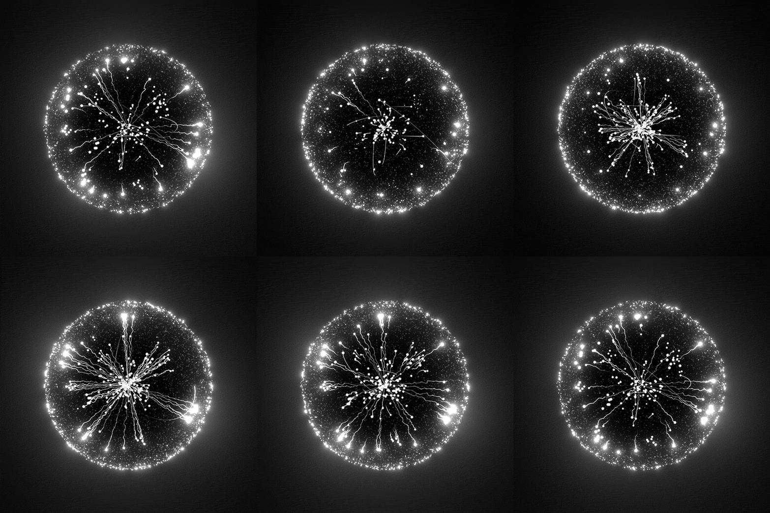
zoofs is a Python library for performing feature selection using a variety of nature inspired wrapper algorithms. The algorithms range from swarm-intelligence to physics based to Evolutionary.
It's an easy to use, flexible and powerful tool to reduce your feature size.
🌟 Like this Project? Give us a star !
📘 Documentation
https://jaswinder9051998.github.io/zoofs/
🔗 Whats new in V0.1.24
- pass kwargs through objective function
- improved logger for results
- added harris hawk algorithm
- now you can pass
timeoutas a parameter to stop operation after the given number of second(s). An amazing alternative to passing number of iterations - Feature score hashing of visited feature sets to increase the overall performance
🛠 Installation
Using pip
Use the package manager to install zoofs.
pip install zoofs
📜 Available Algorithms
| Algorithm Name | Class Name | Description | References doi |
|---|---|---|---|
| Particle Swarm Algorithm | ParticleSwarmOptimization | Utilizes swarm behaviour | https://doi.org/10.1007/978-3-319-13563-2_51 |
| Grey Wolf Algorithm | GreyWolfOptimization | Utilizes wolf hunting behaviour | https://doi.org/10.1016/j.neucom.2015.06.083 |
| Dragon Fly Algorithm | DragonFlyOptimization | Utilizes dragonfly swarm behaviour | https://doi.org/10.1016/j.knosys.2020.106131 |
| Harris Hawk Algorithm | HarrisHawkOptimization | Utilizes hawk hunting behaviour | https://link.springer.com/chapter/10.1007/978-981-32-9990-0_12 |
| Genetic Algorithm Algorithm | GeneticOptimization | Utilizes genetic mutation behaviour | https://doi.org/10.1109/ICDAR.2001.953980 |
| Gravitational Algorithm | GravitationalOptimization | Utilizes newtons gravitational behaviour | https://doi.org/10.1109/ICASSP.2011.5946916 |
More algos soon, stay tuned !
⚡️ Usage
Define your own objective function for optimization !
Classification Example
from sklearn.metrics import log_loss
# define your own objective function, make sure the function receives four parameters,
#  fit your model and return the objective value !
def objective_function_topass(model,X_train, y_train, X_valid, y_valid):
    model.fit(X_train,y_train)
    P=log_loss(y_valid,model.predict_proba(X_valid))
    return P

# import an algorithm !
from zoofs import ParticleSwarmOptimization
# create object of algorithm
algo_object=ParticleSwarmOptimization(objective_function_topass,n_iteration=20,
                                       population_size=20,minimize=True)
import lightgbm as lgb
lgb_model = lgb.LGBMClassifier()
# fit the algorithm
algo_object.fit(lgb_model,X_train, y_train, X_valid, y_valid,verbose=True)
#plot your results
algo_object.plot_history()
Regression Example
from sklearn.metrics import mean_squared_error
# define your own objective function, make sure the function receives four parameters,
#  fit your model and return the objective value !
def objective_function_topass(model,X_train, y_train, X_valid, y_valid):
    model.fit(X_train,y_train)
    P=mean_squared_error(y_valid,model.predict(X_valid))
    return P

# import an algorithm !
from zoofs import ParticleSwarmOptimization
# create object of algorithm
algo_object=ParticleSwarmOptimization(objective_function_topass,n_iteration=20,
                                       population_size=20,minimize=True)
import lightgbm as lgb
lgb_model = lgb.LGBMRegressor()
# fit the algorithm
algo_object.fit(lgb_model,X_train, y_train, X_valid, y_valid,verbose=True)
#plot your results
algo_object.plot_history()
Suggestions for Usage
- As available algorithms are wrapper algos, it is better to use ml models that build quicker, e.g lightgbm, catboost.
- Take sufficient amount for 'population_size' , as this will determine the extent of exploration and exploitation of the algo.
- Ensure that your ml model has its hyperparamters optimized before passing it to zoofs algos.
objective score plot
Algorithms
<details> <summary markdown="span"> Particle Swarm Algorithm </summary>
In computational science, particle swarm optimization (PSO) is a computational method that optimizes a problem by iteratively trying to improve a candidate solution with regard to a given measure of quality. It solves a problem by having a population of candidate solutions, here dubbed particles, and moving these particles around in the search-space according to simple mathematical formula over the particle's position and velocity. Each particle's movement is influenced by its local best known position, but is also guided toward the best known positions in the search-space, which are updated as better positions are found by other particles. This is expected to move the swarm toward the best solutions.
class zoofs.ParticleSwarmOptimization(objective_function,n_iteration=50,population_size=50,minimize=True,c1=2,c2=2,w=0.9)
| Parameters | objective_function : user made function of the signature 'func(model,X_train,y_train,X_test,y_test)'. <br/> <dl> <dd> The function must return a value, that needs to be minimized/maximized. </dd> </dl> n_iteration : int, default=1000 <br/> <dl> <dd> Number of time the algorithm will run </dd> </dl> timeout: int = None <br/> <dl> <dd> Stop operation after the given number of second(s). If this argument is set to None, the operation is executed without time limitation and n_iteration is followed </dd> </dl> population_size : int, default=50 <br/> <dl> <dd> Total size of the population </dd> </dl> minimize : bool, default=True <br/> <dl> <dd> Defines if the objective value is to be maximized or minimized </dd> </dl> c1 : float, default=2.0 <br/> <dl> <dd> first acceleration coefficient of particle swarm </dd> </dl> c2 : float, default=2.0 <br/> <dl> <dd> second acceleration coefficient of particle swarm </dd> </dl> w : float, default=0.9 <br/> <dl> <dd> weight parameter </dd> </dl> |
| Attributes | best_feature_list : array-like <br/> <dl> <dd> Final best set of features </dd> </dl> |
Methods
| Methods | Class Name |
|---|---|
| fit | Run the algorithm |
| plot_history | Plot results achieved across iteration |
fit(model,X_train, y_train, X_test, y_test,verbose=True)
| Parameters | model : <br/> <dl> <dd> machine learning model's object </dd> </dl> X_train : pandas.core.frame.DataFrame of shape (n_samples, n_features) <br/><dl> <dd> Training input samples to be used for machine learning model </dd> </dl> y_train : pandas.core.frame.DataFrame or pandas.core.series.Series of shape (n_samples) <br/> <dl> <dd> The target values (class labels in classification, real numbers in regression). </dd> </dl> X_valid : pandas.core.frame.DataFrame of shape (n_samples, n_features) <br/> <dl> <dd> Validation input samples </dd> </dl> y_valid : pandas.core.frame.DataFrame or pandas.core.series.Series of shape (n_samples) <br/> <dl> <dd> The Validation target values . </dd> </dl> verbose : bool,default=True <br/> <dl> <dd> Print results for iterations </dd> </dl> |
| Returns | best_feature_list : array-like <br/> <dl> <dd> Final best set of features </dd> </dl> |
plot_history()
Plot results across iterations
Example
from sklearn.metrics import log_loss
# define your own objective function, make sure the function receives four parameters,
#  fit your model and return the objective value !
def objective_function_topass(model,X_train, y_train, X_valid, y_valid):
    model.fit(X_train,y_train)
    P=log_loss(y_valid,model.predict_proba(X_valid))
    return P

# import an algorithm !
from zoofs import ParticleSwarmOptimization
# create object of algorithm
algo_object=ParticleSwarmOptimization(objective_function_topass,n_iteration=20,
                                       population_size=20,minimize=True,c1=2,c2=2,w=0.9)
import lightgbm as lgb
lgb_model = lgb.LGBMClassifier()
# fit the algorithm
algo_object.fit(lgb_model,X_train, y_train, X_valid, y_valid,verbose=True)
#plot your results
algo_object.plot_history()

The Grey Wolf Optimizer (GWO) mimics the leadership hierarchy and hunting mechanism of grey wolves in nature. Four types of grey wolves such as alpha, beta, delta, and omega are employed for simulating the leadership hierarchy. In addition, three main steps of hunting, searching for prey, encircling prey, and attacking prey, are implemented to perform optimization.
class zoofs.GreyWolfOptimization(objective_function,n_iteration=50,population_size=50,minimize=True)
| Parameters | objective_function : user made function of the signature 'func(model,X_train,y_train,X_test,y_test)'. <br/> <dl> <dd> The function must return a value, that needs to be minimized/maximized. </dd> </dl> n_iteration : int, default=50 <br/> <dl> <dd> Number of time the algorithm will run </dd> </dl> timeout: int = None <br/> <dl> <dd> Stop operation after the given number of second(s). If this argument is set to None, the operation is executed without time limitation and n_iteration is followed </dd> </dl> population_size : int, default=50 <br/> <dl> <dd> Total size of the population </dd> </dl> method : {1, 2}, default=1 <br/> <dl> <dd> Choose the between the two methods of grey wolf optimization </dd> </dl> minimize : bool, default=True <br/> <dl> <dd> Defines if the objective value is to be maximized or minimized </dd> </dl> |
| Attributes | best_feature_list : array-like <br/> <dl> <dd> Final best set of features </dd> </dl> |
Methods
| Methods | Class Name |
|---|---|
| fit | Run the algorithm |
| plot_history | Plot results achieved across iteration |
fit(model,X_train,y_train,X_valid,y_valid,method=1,verbose=True)
| Parameters | model : <br/> <dl> <dd> machine learning model's object </dd> </dl> X_train : pandas.core.frame.DataFrame of shape (n_samples, n_features) <br/><dl> <dd> Training input samples to be used for machine learning model </dd> </dl> y_train : pandas.core.frame.DataFrame or pandas.core.series.Series of shape (n_samples) <br/> <dl> <dd> The target values (class labels in classification, real numbers in regression). </dd> </dl> X_valid : pandas.core.frame.DataFrame of shape (n_samples, n_features) <br/> <dl> <dd> Validation input samples </dd> </dl> y_valid : pandas.core.frame.DataFrame or pandas.core.series.Series of shape (n_samples) <br/> <dl> <dd> The Validation target values . </dd> </dl> verbose : bool,default=True <br/> <dl> <dd> Print results for iterations </dd> </dl> |
| Returns | best_feature_list : array-like <br/> <dl> <dd> Final best set of features </dd> </dl> |
plot_history()
Plot results across iterations
Example
from sklearn.metrics import log_loss
# define your own objective function, make sure the function receives four parameters,
#  fit your model and return the objective value !
def objective_function_topass(model,X_train, y_train, X_valid, y_valid):
    model.fit(X_train,y_train)
    P=log_loss(y_valid,model.predict_proba(X_valid))
    return P

# import an algorithm !
from zoofs import GreyWolfOptimization
# create object of algorithm
algo_object=GreyWolfOptimization(objective_function_topass,n_iteration=20,method=1,
                                    population_size=20,minimize=True)
import lightgbm as lgb
lgb_model = lgb.LGBMClassifier()
# fit the algorithm
algo_object.fit(lgb_model,X_train, y_train, X_valid, y_valid,verbose=True)
#plot your results
algo_object.plot_history()

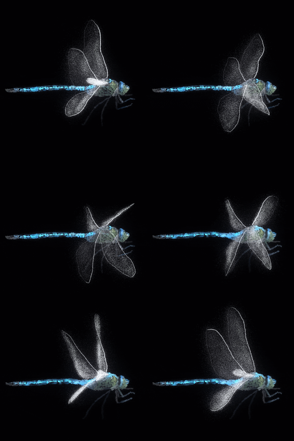
The main inspiration of the Dragonfly Algorithm (DA) algorithm originates from static and dynamic swarming behaviours. These two swarming behaviours are very similar to the two main phases of optimization using meta-heuristics: exploration and exploitation. Dragonflies create sub swarms and fly over different areas in a static swarm, which is the main objective of the exploration phase. In the static swarm, however, dragonflies fly in bigger swarms and along one direction, which is favourable in the exploitation phase.
class zoofs.DragonFlyOptimization(objective_function,n_iteration=50,population_size=50,minimize=True)
| Parameters | objective_function : user made function of the signature 'func(model,X_train,y_train,X_test,y_test)'. <br/> <dl> <dd> The function must return a value, that needs to be minimized/maximized. </dd> </dl> n_iteration : int, default=50 <br/> <dl> <dd> Number of time the algorithm will run </dd> </dl> timeout: int = None <br/> <dl> <dd> Stop operation after the given number of second(s). If this argument is set to None, the operation is executed without time limitation and n_iteration is followed </dd> </dl> population_size : int, default=50 <br/> <dl> <dd> Total size of the population </dd> </dl> method : {'linear','random','quadraic','sinusoidal'}, default='sinusoidal' <br/> <dl> <dd> Choose the between the three methods of Dragon Fly optimization </dd> </dl> minimize : bool, default=True <br/> <dl> <dd> Defines if the objective value is to be maximized or minimized </dd> </dl> |
| Attributes | best_feature_list : array-like <br/> <dl> <dd> Final best set of features </dd> </dl> |
Methods
| Methods | Class Name |
|---|---|
| fit | Run the algorithm |
| plot_history | Plot results achieved across iteration |
fit(model,X_train,y_train,X_valid,y_valid,method='sinusoidal',verbose=True)
| Parameters | model : <br/> <dl> <dd> machine learning model's object </dd> </dl> X_train : pandas.core.frame.DataFrame of shape (n_samples, n_features) <br/><dl> <dd> Training input samples to be used for machine learning model </dd> </dl> y_train : pandas.core.frame.DataFrame or pandas.core.series.Series of shape (n_samples) <br/> <dl> <dd> The target values (class labels in classification, real numbers in regression). </dd> </dl> X_valid : pandas.core.frame.DataFrame of shape (n_samples, n_features) <br/> <dl> <dd> Validation input samples </dd> </dl> y_valid : pandas.core.frame.DataFrame or pandas.core.series.Series of shape (n_samples) <br/> <dl> <dd> The Validation target values . </dd> </dl> verbose : bool,default=True <br/> <dl> <dd> Print results for iterations </dd> </dl> |
| Returns | best_feature_list : array-like <br/> <dl> <dd> Final best set of features </dd> </dl> |
plot_history()
Plot results across iterations
Example
from sklearn.metrics import log_loss
# define your own objective function, make sure the function receives four parameters,
#  fit your model and return the objective value !
def objective_function_topass(model,X_train, y_train, X_valid, y_valid):
    model.fit(X_train,y_train)
    P=log_loss(y_valid,model.predict_proba(X_valid))
    return P

# import an algorithm !
from zoofs import DragonFlyOptimization
# create object of algorithm
algo_object=DragonFlyOptimization(objective_function_topass,n_iteration=20,method='sinusoidal',
                                    population_size=20,minimize=True)
import lightgbm as lgb
lgb_model = lgb.LGBMClassifier()
# fit the algorithm
algo_object.fit(lgb_model,X_train, y_train, X_valid, y_valid,  verbose=True)
#plot your results
algo_object.plot_history()

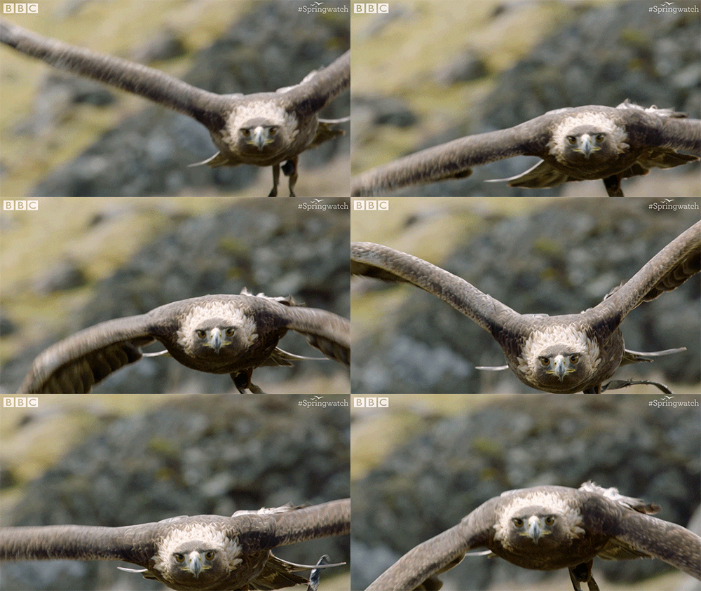
HHO is a popular swarm-based, gradient-free optimization algorithm with several active and time-varying phases of exploration and exploitation. This algorithm initially published by the prestigious Journal of Future Generation Computer Systems (FGCS) in 2019, and from the first day, it has gained increasing attention among researchers due to its flexible structure, high performance, and high-quality results. The main logic of the HHO method is designed based on the cooperative behaviour and chasing styles of Harris' hawks in nature called "surprise pounce". Currently, there are many suggestions about how to enhance the functionality of HHO, and there are also several enhanced variants of the HHO in the leading Elsevier and IEEE transaction journals.
class zoofs.HarrisHawkOptimization(objective_function,n_iteration=50,population_size=50,minimize=True,beta=0.5)
| Parameters | objective_function : user made function of the signature 'func(model,X_train,y_train,X_test,y_test)'. <br/> <dl> <dd> The function must return a value, that needs to be minimized/maximized. </dd> </dl> n_iteration : int, default=1000 <br/> <dl> <dd> Number of time the algorithm will run </dd> </dl> timeout: int = None <br/> <dl> <dd> Stop operation after the given number of second(s). If this argument is set to None, the operation is executed without time limitation and n_iteration is followed </dd> </dl> population_size : int, default=50 <br/> <dl> <dd> Total size of the population </dd> </dl> minimize : bool, default=True <br/> <dl> <dd> Defines if the objective value is to be maximized or minimized </dd> </dl> beta : float, default=0.5 <br/> <dl> <dd> value for levy random walk </dd> </dl> |
| Attributes | best_feature_list : array-like <br/> <dl> <dd> Final best set of features </dd> </dl> |
Methods
| Methods | Class Name |
|---|---|
| fit | Run the algorithm |
| plot_history | Plot results achieved across iteration |
fit(model,X_train, y_train, X_test, y_test,verbose=True)
| Parameters | model : <br/> <dl> <dd> machine learning model's object </dd> </dl> X_train : pandas.core.frame.DataFrame of shape (n_samples, n_features) <br/><dl> <dd> Training input samples to be used for machine learning model </dd> </dl> y_train : pandas.core.frame.DataFrame or pandas.core.series.Series of shape (n_samples) <br/> <dl> <dd> The target values (class labels in classification, real numbers in regression). </dd> </dl> X_valid : pandas.core.frame.DataFrame of shape (n_samples, n_features) <br/> <dl> <dd> Validation input samples </dd> </dl> y_valid : pandas.core.frame.DataFrame or pandas.core.series.Series of shape (n_samples) <br/> <dl> <dd> The Validation target values . </dd> </dl> verbose : bool,default=True <br/> <dl> <dd> Print results for iterations </dd> </dl> |
| Returns | best_feature_list : array-like <br/> <dl> <dd> Final best set of features </dd> </dl> |
plot_history()
Plot results across iterations
Example
from sklearn.metrics import log_loss
# define your own objective function, make sure the function receives four parameters,
#  fit your model and return the objective value !
def objective_function_topass(model,X_train, y_train, X_valid, y_valid):
    model.fit(X_train,y_train)
    P=log_loss(y_valid,model.predict_proba(X_valid))
    return P

# import an algorithm !
from zoofs import HarrisHawkOptimization
# create object of algorithm
algo_object=HarrisHawkOptimization(objective_function_topass,n_iteration=20,
                                       population_size=20,minimize=True)
import lightgbm as lgb
lgb_model = lgb.LGBMClassifier()
# fit the algorithm
algo_object.fit(lgb_model,X_train, y_train, X_valid, y_valid,verbose=True)
#plot your results
algo_object.plot_history()

In computer science and operations research, a genetic algorithm (GA) is a metaheuristic inspired by the process of natural selection that belongs to the larger class of evolutionary algorithms (EA). Genetic algorithms are commonly used to generate high-quality solutions to optimization and search problems by relying on biologically inspired operators such as mutation, crossover and selection. Some examples of GA applications include optimizing decision trees for better performance, automatically solve sudoku puzzles, hyperparameter optimization, etc.
class zoofs.GeneticOptimization(objective_function,n_iteration=20,population_size=20,selective_pressure=2,elitism=2,mutation_rate=0.05,minimize=True)
| Parameters | objective_function : user made function of the signature 'func(model,X_train,y_train,X_test,y_test)'. <br/> <dl> <dd> The function must return a value, that needs to be minimized/maximized. </dd> </dl> n_iteration: int, default=50 <br/> <dl> <dd> Number of time the algorithm will run </dd> </dl> timeout: int = None <br/> <dl> <dd> Stop operation after the given number of second(s). If this argument is set to None, the operation is executed without time limitation and n_iteration is followed </dd> </dl> population_size : int, default=50 <br/> <dl> <dd> Total size of the population </dd> </dl> selective_pressure: int, default=2 <br/> <dl> <dd>measure of reproductive opportunities for each organism in the population </dd> </dl> elitism: int, default=2 <br/> <dl> <dd> number of top individuals to be considered as elites </dd> </dl> mutation_rate: float, default=0.05 <br/> <dl> <dd> rate of mutation in the population's gene </dd> </dl> minimize: bool, default=True <br/> <dl> <dd> Defines if the objective value is to be maximized or minimized </dd> </dl> |
| Attributes | best_feature_list : array-like <br/> <dl> <dd> Final best set of features </dd> </dl> |
Methods
| Methods | Class Name |
|---|---|
| fit | Run the algorithm |
| plot_history | Plot results achieved across iteration |
fit(model,X_train,y_train,X_valid,y_valid,verbose=True)
| Parameters | model : <br/> <dl> <dd> machine learning model's object </dd> </dl> X_train : pandas.core.frame.DataFrame of shape (n_samples, n_features) <br/><dl> <dd> Training input samples to be used for machine learning model </dd> </dl> y_train : pandas.core.frame.DataFrame or pandas.core.series.Series of shape (n_samples) <br/> <dl> <dd> The target values (class labels in classification, real numbers in regression). </dd> </dl> X_valid : pandas.core.frame.DataFrame of shape (n_samples, n_features) <br/> <dl> <dd> Validation input samples </dd> </dl> y_valid : pandas.core.frame.DataFrame or pandas.core.series.Series of shape (n_samples) <br/> <dl> <dd> The Validation target values . </dd> </dl> verbose : bool,default=True <br/> <dl> <dd> Print results for iterations </dd> </dl> |
| Returns | best_feature_list : array-like <br/> <dl> <dd> Final best set of features </dd> </dl> |
plot_history()
Plot results across iterations
Example
from sklearn.metrics import log_loss
# define your own objective function, make sure the function receives four parameters,
#  fit your model and return the objective value !
def objective_function_topass(model,X_train, y_train, X_valid, y_valid):
    model.fit(X_train,y_train)
    P=log_loss(y_valid,model.predict_proba(X_valid))
    return P

# import an algorithm !
from zoofs import GeneticOptimization
# create object of algorithm
algo_object=GeneticOptimization(objective_function_topass,n_iteration=20,
                            population_size=20,selective_pressure=2,elitism=2,
                            mutation_rate=0.05,minimize=True)
import lightgbm as lgb
lgb_model = lgb.LGBMClassifier()
# fit the algorithm
algo_object.fit(lgb_model,X_train, y_train,X_valid, y_valid, verbose=True)
#plot your results
algo_object.plot_history()

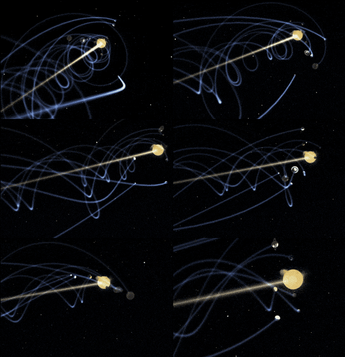
Gravitational Algorithm is based on the law of gravity and mass interactions is introduced. In the algorithm, the searcher agents are a collection of masses which interact with each other based on the Newtonian gravity and the laws of motion.
class zoofs.GravitationalOptimization(self,objective_function,n_iteration=50,population_size=50,g0=100,eps=0.5,minimize=True)
| Parameters | objective_function : user made function of the signature 'func(model,X_train,y_train,X_test,y_test)'. <br/> <dl> <dd> The function must return a value, that needs to be minimized/maximized. </dd> </dl> n_iteration: int, default=50 <br/> <dl> <dd> Number of time the algorithm will run </dd> </dl> timeout: int = None <br/> <dl> <dd> Stop operation after the given number of second(s). If this argument is set to None, the operation is executed without time limitation and n_iteration is followed </dd> </dl> population_size : int, default=50 <br/> <dl> <dd> Total size of the population </dd> </dl> g0: float, default=100 <br/> <dl> <dd> gravitational strength constant </dd> </dl> eps: float, default=0.5 <br/> <dl> <dd> distance constant </dd> </dl>minimize: bool, default=True <br/> <dl> <dd> Defines if the objective value is to be maximized or minimized </dd> </dl> |
| Attributes | best_feature_list : array-like <br/> <dl> <dd> Final best set of features </dd> </dl> |
Methods
| Methods | Class Name |
|---|---|
| fit | Run the algorithm |
| plot_history | Plot results achieved across iteration |
fit(model,X_train,y_train,X_valid,y_valid,verbose=True)
| Parameters | model : <br/> <dl> <dd> machine learning model's object </dd> </dl> X_train : pandas.core.frame.DataFrame of shape (n_samples, n_features) <br/><dl> <dd> Training input samples to be used for machine learning model </dd> </dl> y_train : pandas.core.frame.DataFrame or pandas.core.series.Series of shape (n_samples) <br/> <dl> <dd> The target values (class labels in classification, real numbers in regression). </dd> </dl> X_valid : pandas.core.frame.DataFrame of shape (n_samples, n_features) <br/> <dl> <dd> Validation input samples </dd> </dl> y_valid : pandas.core.frame.DataFrame or pandas.core.series.Series of shape (n_samples) <br/> <dl> <dd> The Validation target values . </dd> </dl> verbose : bool,default=True <br/> <dl> <dd> Print results for iterations </dd> </dl> |
| Returns | best_feature_list : array-like <br/> <dl> <dd> Final best set of features </dd> </dl> |
plot_history()
Plot results across iterations
Example
from sklearn.metrics import log_loss
# define your own objective function, make sure the function receives four parameters,
#  fit your model and return the objective value !
def objective_function_topass(model,X_train, y_train, X_valid, y_valid):
    model.fit(X_train,y_train)
    P=log_loss(y_valid,model.predict_proba(X_valid))
    return P

# import an algorithm !
from zoofs import GravitationalOptimization
# create object of algorithm
algo_object=GravitationalOptimization(objective_function_topass,n_iteration=50,
                                population_size=50,g0=100,eps=0.5,minimize=True)
import lightgbm as lgb
lgb_model = lgb.LGBMClassifier()
# fit the algorithm
algo_object.fit(lgb_model,X_train, y_train, X_valid, y_valid, verbose=True)
#plot your results
algo_object.plot_history()
Support zoofs
The development of zoofs relies completely on contributions.
Contributing
Pull requests are welcome. For major changes, please open an issue first to discuss what you would like to change.
Please make sure to update tests as appropriate.
First roll out
18,08,2021
