Awesome
ERAN <img width="100" alt="portfolio_view" align="right" src="http://safeai.ethz.ch/img/sri-logo.svg">
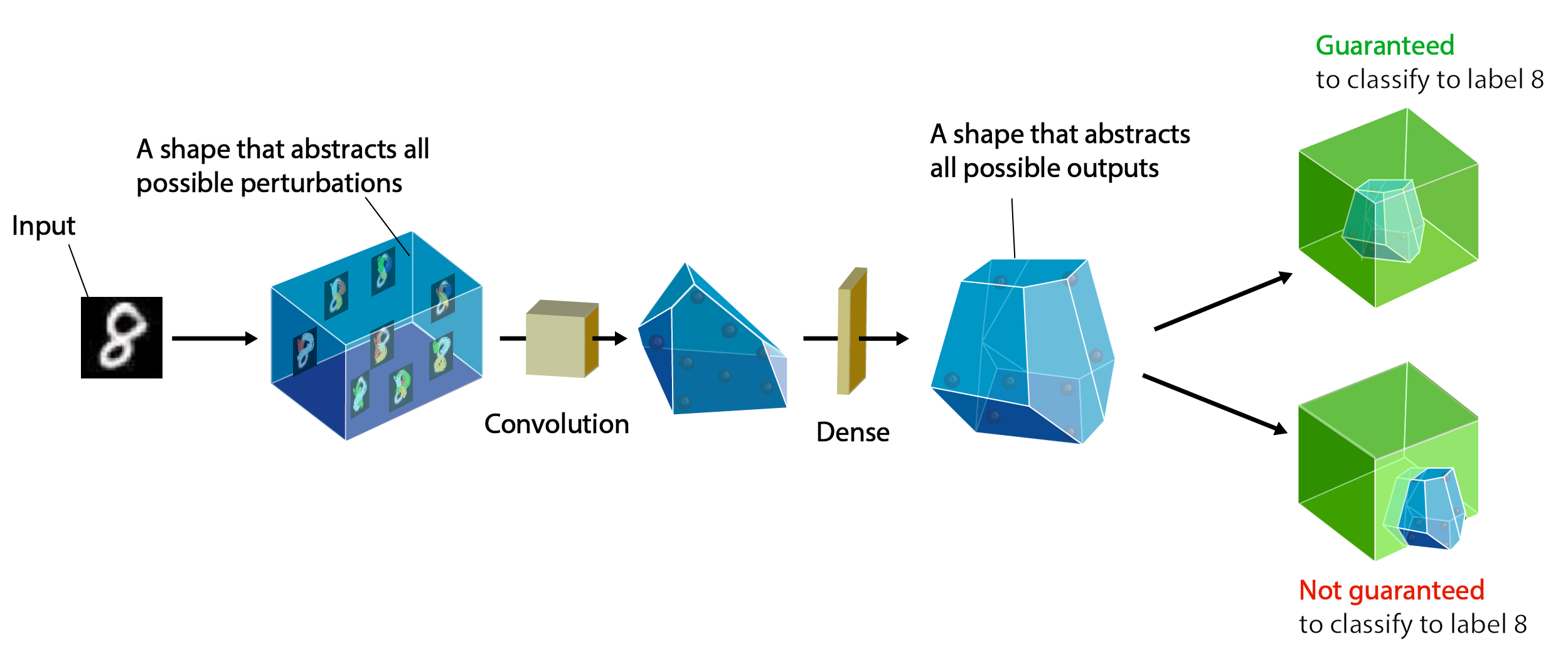
ETH Robustness Analyzer for Neural Networks (ERAN) is a state-of-the-art sound, precise, scalable, and extensible analyzer based on abstract interpretation for the complete and incomplete verification of MNIST, CIFAR10, and ACAS Xu based networks. ERAN produces state-of-the-art precision and performance for both complete and incomplete verification and can be tuned to provide best precision and scalability (see recommended configuration settings at the bottom). ERAN is developed at the SRI Lab, Department of Computer Science, ETH Zurich as part of the Safe AI project. The goal of ERAN is to automatically verify safety properties of neural networks with feedforward, convolutional, and residual layers against input perturbations (e.g., L∞-norm attacks, geometric transformations, vector field deformations, etc).
ERAN combines abstract domains with custom multi-neuron relaxations from PRIMA to support fully-connected, convolutional, and residual networks with ReLU, Sigmoid, Tanh, and Maxpool activations. ERAN is sound under floating point arithmetic with the exception of the (MI)LP solver used in RefineZono and RefinePoly. The employed abstract domains are specifically designed for the setting of neural networks and aim to balance scalability and precision. Specifically, ERAN supports the following analysis:
-
DeepZ [NIPS'18]: contains specialized abstract Zonotope transformers for handling ReLU, Sigmoid and Tanh activation functions.
-
DeepPoly [POPL'19]: based on a domain that combines floating point Polyhedra with Intervals.
-
GPUPoly [MLSys'2021]: leverages an efficient GPU implementation to scale DeepPoly to much larger networks.
-
RefineZono [ICLR'19]: combines DeepZ analysis with MILP and LP solvers for more precision.
-
RefinePoly/RefineGPUPoly [NeurIPS'19]: combines DeepPoly/GPUPoly analysis with (MI)LP refinement and PRIMA framework [arXiv'2021] to compute group-wise joint neuron abstractions for state-of-the-art precision and scalability.
All analysis are implemented using the ELINA library for numerical abstractions. More details can be found in the publications below.
ERAN vs AI2
Note that ERAN subsumes the first abstract interpretation based analyzer AI2, so if you aim to compare, please use ERAN as a baseline.
USER MANUAL
For a detailed desciption of the options provided and the implentation of ERAN, you can download the user manual.
Requirements
GNU C compiler, ELINA, Gurobi's Python interface,
python3.6 or higher, tensorflow 1.11 or higher, numpy.
Installation
Clone the ERAN repository via git as follows:
git clone https://github.com/eth-sri/ERAN.git
cd ERAN
The dependencies for ERAN can be installed step by step as follows (sudo rights might be required):
Note that it might be required to use sudo -E to for the right environment variables to be set.
Ensure that the following tools are available before using the install script:
- cmake (>=3.17.1),
- m4 (>=1.4.18)
- autoconf,
- libtool,
- pdftex.
On Ubuntu systems they can be installed using:
sudo apt-get install m4
sudo apt-get install build-essential
sudo apt-get install autoconf
sudo apt-get install libtool
sudo apt-get install texlive-latex-base
Consult https://cmake.org/cmake/help/latest/command/install.html for the install of cmake or use:
wget https://github.com/Kitware/CMake/releases/download/v3.19.7/cmake-3.19.7-Linux-x86_64.sh
sudo bash ./cmake-3.19.7-Linux-x86_64.sh
sudo rm /usr/bin/cmake
sudo ln -s ./cmake-3.19.7-Linux-x86_64/bin/cmake /usr/bin/cmake
The steps following from here can be done automatically using sudo bash ./install.sh
Install gmp:
wget https://gmplib.org/download/gmp/gmp-6.1.2.tar.xz
tar -xvf gmp-6.1.2.tar.xz
cd gmp-6.1.2
./configure --enable-cxx
make
make install
cd ..
rm gmp-6.1.2.tar.xz
Install mpfr:
wget https://files.sri.inf.ethz.ch/eran/mpfr/mpfr-4.1.0.tar.xz
tar -xvf mpfr-4.1.0.tar.xz
cd mpfr-4.1.0
./configure
make
make install
cd ..
rm mpfr-4.1.0.tar.xz
Install cddlib:
wget https://github.com/cddlib/cddlib/releases/download/0.94m/cddlib-0.94m.tar.gz
tar zxf cddlib-0.94m.tar.gz
rm cddlib-0.94m.tar.gz
cd cddlib-0.94m
./configure
make
make install
cd ..
Install Gurobi:
wget https://packages.gurobi.com/9.1/gurobi9.1.2_linux64.tar.gz
tar -xvf gurobi9.1.2_linux64.tar.gz
cd gurobi912/linux64/src/build
sed -ie 's/^C++FLAGS =.*$/& -fPIC/' Makefile
make
cp libgurobi_c++.a ../../lib/
cd ../../
cp lib/libgurobi91.so /usr/local/lib
python3 setup.py install
cd ../../
Update environment variables:
export GUROBI_HOME="$PWD/gurobi912/linux64"
export PATH="$PATH:${GUROBI_HOME}/bin"
export CPATH="$CPATH:${GUROBI_HOME}/include"
export LD_LIBRARY_PATH=$LD_LIBRARY_PATH:/usr/local/lib:${GUROBI_HOME}/lib
Install ELINA:
git clone https://github.com/eth-sri/ELINA.git
cd ELINA
./configure -use-deeppoly -use-gurobi -use-fconv -use-cuda
cd ./gpupoly/
cmake .
cd ..
make
make install
cd ..
Install DeepG (note that with an already existing version of ERAN you have to start at step Install Gurobi):
git clone https://github.com/eth-sri/deepg.git
cd deepg/code
mkdir build
make shared_object
cp ./build/libgeometric.so /usr/lib
cd ../..
We also provide scripts that will install ELINA and all the necessary dependencies. One can run it as follows (remove the -use-cuda argument on machines without GPU):
sudo ./install.sh -use-cuda
source gurobi_setup_path.sh
Note that to run ERAN with Gurobi one needs to obtain an academic license for gurobi from https://user.gurobi.com/download/licenses/free-academic. If you plan on running ERAN on Windows WSL2, you might prefer requesting a cloud-based academic license at https://license.gurobi.com, in order to avoid this issue with early-expiring licenses.
To install the remaining python dependencies (numpy and tensorflow), type:
pip3 install -r requirements.txt
ERAN may not be compatible with older versions of tensorflow (we have tested ERAN with versions >= 1.11.0), so if you have an older version and want to keep it, then we recommend using the python virtual environment for installing tensorflow.
If gurobipy is not found despite executing python setup.py install in the corresponding gurobi directory,
gurobipy can alternatively be installed using conda with:
conda config --add channels http://conda.anaconda.org/gurobi
conda install gurobi
Usage
cd tf_verify

python3 . --netname <path to the network file> --epsilon <float between 0 and 1> --domain <deepzono/deeppoly/refinezono/refinepoly> --dataset <mnist/cifar10/acasxu> --zonotope <path to the zonotope specfile>  [optional] --complete <True/False> --timeout_complete <float> --timeout_lp <float> --timeout_milp <float> --use_area_heuristic <True/False> --mean <float(s)> --std <float(s)> --use_milp <True/False> --use_2relu --use_3relu --dyn_krelu --numproc <int>
-
<epsilon>: specifies bound for the L∞-norm based perturbation (default is 0). This parameter is not required for testing ACAS Xu networks. -
<zonotope>: The Zonotope specification file can be comma or whitespace separated file where the first two integers can specify the number of input dimensions D and the number of error terms per dimension N. The following D*N doubles specify the coefficient of error terms. For every dimension i, the error terms are numbered from 0 to N-1 where the 0-th error term is the central error term. See an example here [https://github.com/eth-sri/eran/files/3653882/zonotope_example.txt]. This option only works with the "deepzono" or "refinezono" domain. -
<use_area_heuristic>: specifies whether to use area heuristic for the ReLU approximation in DeepPoly (default is true). -
<mean>: specifies mean used to normalize the data. If the data has multiple channels the mean for every channel has to be provided (e.g. for cifar10 --mean 0.485, 0.456, 0.406) (default is 0 for non-geometric mnist and 0.5 0.5 0.5 otherwise) -
<std>: specifies standard deviation used to normalize the data. If the data has multiple channels the standard deviaton for every channel has to be provided (e.g. for cifar10 --std 0.2 0.3 0.2) (default is 1 1 1) -
<use_milp>: specifies whether to use MILP (default is true). -
<sparse_n>: specifies the size of "k" for the kReLU framework (default is 70). -
<numproc>: specifies how many processes to use for MILP, LP and k-ReLU (default is the number of processors in your machine). -
<geometric>: specifies whether to do geometric analysis (default is false). -
<geometric_config>: specifies the geometric configuration file location. -
<data_dir>: specifies the geometric data location. -
<num_params>: specifies the number of transformation parameters (default is 0) -
<attack>: specifies whether to verify attack images (default is false). -
<specnumber>: the property number for the ACASXu networks -
Refinezono and RefinePoly refines the analysis results from the DeepZ and DeepPoly domain respectively using the approach in our ICLR'19 paper. The optional parameters timeout_lp and timeout_milp (default is 1 sec for both) specify the timeouts for the LP and MILP forumlations of the network respectively.
-
Since Refinezono and RefinePoly uses timeout for the gurobi solver, the results will vary depending on the processor speeds.
-
Setting the parameter "complete" (default is False) to True will enable MILP based complete verification using the bounds provided by the specified domain.
-
When ERAN fails to prove the robustness of a given network in a specified region, it searches for an adversarial example and prints an adversarial image within the specified adversarial region along with the misclassified label and the correct label. ERAN does so for both complete and incomplete verification.
Example
L_oo Specification
python3 . --netname ../nets/onnx/mnist/convBig__DiffAI.onnx --epsilon 0.1 --domain deepzono --dataset mnist
will evaluate the local robustness of the MNIST convolutional network (upto 35K neurons) with ReLU activation trained using DiffAI on the 100 MNIST test images. In the above setting, epsilon=0.1 and the domain used by our analyzer is the deepzono domain. Our analyzer will print the following:
-
'Verified safe' for an image when it can prove the robustness of the network
-
'Verified unsafe' for an image for which it can provide a concrete adversarial example
-
'Failed' when it cannot.
-
It will also print an error message when the network misclassifies an image.
-
the timing in seconds.
-
The ratio of images on which the network is robust versus the number of images on which it classifies correctly.
Zonotope Specification
python3 . --netname ../nets/onnx/mnist/convBig__DiffAI.onnx --zonotope some_path/zonotope_example.txt --domain deepzono
will check if the Zonotope specification specified in "zonotope_example" holds for the network and will output "Verified safe", "Verified unsafe" or "Failed" along with the timing.
Similarly, for the ACAS Xu networks, ERAN will output whether the property has been verified along with the timing.
ACASXu Specification
python3 . --netname ../data/acasxu/nets/ACASXU_run2a_3_3_batch_2000.onnx --dataset acasxu --domain deepzono --specnumber 9
will run DeepZ for analyzing property 9 of ACASXu benchmarks. The ACASXU networks are in data/acasxu/nets directory and the one chosen for a given property is defined in the Reluplex paper.
Geometric analysis
python3 . --netname ../nets/onnx/mnist/convBig__DiffAI.onnx --geometric --geometric_config ../deepg/code/examples/example1/config.txt --num_params 1 --dataset mnist
will on the fly generate geometric perturbed images and evaluate the network against them. For more information on the geometric configuration file please see Format of the configuration file in DeepG.
python3 . --netname ../nets/onnx/mnist/convBig__DiffAI.onnx --geometric --data_dir ../deepg/code/examples/example1/ --num_params 1 --dataset mnist --attack
will evaluate the generated geometric perturbed images in the given data_dir and also evaluate generated attack images.
Recommended Configuration for Scalable Complete Verification
Use the "deeppoly" or "deepzono" domain with "--complete True" option
Recommended Configuration for More Precise but relatively expensive Incomplete Verification
Use the "refinepoly" or if a gpu is available "refinegpupoly" domain with , "--sparse_n 100", and "--timeout_final_lp 100".
For MLPs use "--refine_neurons", "--use_milp True", "--timeout_milp 10", "--timeout_lp 10" to do a neuronweise bound refinement.
For Conv networks use "--partial_milp {1,2}" (choose at most number of linear layers), "--max_milp_neurons 100", and "--timeout_final_milp 250" to use a MILP encoding for the last layers.
Examples:
To certify e.g. CNN-B-ADV introduced as a benchmark for SDP-FO in [1] on the 100 random samples from [2] against L-inf perturbations of magnitude 2/255 use:
python3 . --netname ../nets/CNN_B_CIFAR_ADV.onnx --dataset cifar10 --subset b_adv --domain refinegpupoly --epsilon 0.00784313725 --sparse_n 100 --partial_milp 1 --max_milp_neurons 250 --timeout_final_milp 500 --mean 0.49137255 0.48235294 0.44666667 --std 0.24705882 0.24352941 0.26156863
to certify 43 of the 100 samples as correct with an average runtime of around 260s per sample (including timed out attempts).
Recommended Configuration for Faster but relatively imprecise Incomplete Verification
Use the "deeppoly" or if a gpu is available "gpupoly" domain
Certification of Vector Field Deformations
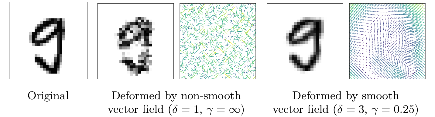
Vector field deformations, which displace pixels instead of directly manipulating pixel values, can be intuitively parametrized by their displacement magnitude delta, i.e., how far every pixel can move, and their smoothness gamma, i.e., how much neighboring displacement vectors can differ from each other (more details can be found in Section 3 of our paper). ERAN can certify both non-smooth vector fields:
python3 . --netname ../nets/onnx/mnist/convBig__DiffAI.onnx --dataset mnist --domain deeppoly --spatial --t-norm inf --delta 0.3
and smooth vector fields:
python3 . --netname ../nets/pytorch/onnx/convBig__DiffAI.onnx --dataset mnist --domain deeppoly --spatial --t-norm inf --delta 0.3 --gamma 0.1
Certification of vector field deformations is compatible with the "deeppoly" and "refinepoly" domains, and can be made more precise with the kReLU framework (e.g., "--use_milp True", "--sparse_n 15", "--refine_neurons", "timeout_milp 10", and "timeout_lp 10") or complete certification ("--complete True").
Publications
-
PRIMA: Precise and General Neural Network Certification via Multi-Neuron Convex Relaxations
Mark Niklas Müller, Gleb Makarchuk, Gagandeep Singh, Markus Püschel, Martin Vechev
POPL 2022.
-
Scaling Polyhedral Neural Network Verification on GPUs
Christoph Müller, Francois Serre, Gagandeep Singh, Markus Puschel, Martin Vechev
MLSys 2021.
-
Efficient Certification of Spatial Robustness
Anian Ruoss, Maximilian Baader, Mislav Balunovic, Martin Vechev
AAAI 2021.
-
Certifying Geometric Robustness of Neural Networks
Mislav Balunovic, Maximilian Baader, Gagandeep Singh, Timon Gehr, Martin Vechev
NeurIPS 2019.
-
Beyond the Single Neuron Convex Barrier for Neural Network Certification.
Gagandeep Singh, Rupanshu Ganvir, Markus Püschel, and Martin Vechev.
NeurIPS 2019.
-
Boosting Robustness Certification of Neural Networks.
Gagandeep Singh, Timon Gehr, Markus Püschel, and Martin Vechev.
ICLR 2019.
-
An Abstract Domain for Certifying Neural Networks.
Gagandeep Singh, Timon Gehr, Markus Püschel, and Martin Vechev.
POPL 2019.
-
Fast and Effective Robustness Certification.
Gagandeep Singh, Timon Gehr, Matthew Mirman, Markus Püschel, and Martin Vechev.
NeurIPS 2018.
Neural Networks and Datasets
We provide a number of pretrained MNIST and CIAFR10 defended and undefended feedforward and convolutional neural networks with ReLU, Sigmoid and Tanh activations trained with the PyTorch and TensorFlow frameworks. The adversarial training to obtain the defended networks is performed using PGD and DiffAI. We report the (maximum) number of activation layers (including MaxPool) of any path through a network.
| Dataset | Model | Type | #units | #activation layers | Activation | Training Defense | Download |
|---|---|---|---|---|---|---|---|
| MNIST | 3x50 | fully connected | 110 | 3 | ReLU | None | :arrow_down: |
| 3x100 | fully connected | 210 | 3 | ReLU | None | :arrow_down: | |
| 5x100 | fully connected | 510 | 6 | ReLU | DiffAI | :arrow_down: | |
| 6x100 | fully connected | 510 | 6 | ReLU | None | :arrow_down: | |
| 9x100 | fully connected | 810 | 9 | ReLU | None | :arrow_down: | |
| 6x200 | fully connected | 1,010 | 6 | ReLU | None | :arrow_down: | |
| 9x200 | fully connected | 1,610 | 9 | ReLU | None | :arrow_down: | |
| 6x500 | fully connected | 3,000 | 6 | ReLU | None | :arrow_down: | |
| 6x500 | fully connected | 3,000 | 6 | ReLU | PGD ε=0.1 | :arrow_down: | |
| 6x500 | fully connected | 3,000 | 6 | ReLU | PGD ε=0.3 | :arrow_down: | |
| 6x500 | fully connected | 3,000 | 6 | Sigmoid | None | :arrow_down: | |
| 6x500 | fully connected | 3,000 | 6 | Sigmoid | PGD ε=0.1 | :arrow_down: | |
| 6x500 | fully connected | 3,000 | 6 | Sigmoid | PGD ε=0.3 | :arrow_down: | |
| 6x500 | fully connected | 3,000 | 6 | Tanh | None | :arrow_down: | |
| 6x500 | fully connected | 3,000 | 6 | Tanh | PGD ε=0.1 | :arrow_down: | |
| 6x500 | fully connected | 3,000 | 6 | Tanh | PGD ε=0.3 | :arrow_down: | |
| 4x1024 | fully connected | 3,072 | 3 | ReLU | None | :arrow_down: | |
| ConvSmall | convolutional | 3,604 | 3 | ReLU | None | :arrow_down: | |
| ConvSmall | convolutional | 3,604 | 3 | ReLU | PGD | :arrow_down: | |
| ConvSmall | convolutional | 3,604 | 3 | ReLU | DiffAI | :arrow_down: | |
| ConvMed | convolutional | 5,704 | 3 | ReLU | None | :arrow_down: | |
| ConvMed | convolutional | 5,704 | 3 | ReLU | PGD ε=0.1 | :arrow_down: | |
| ConvMed | convolutional | 5,704 | 3 | ReLU | PGD ε=0.3 | :arrow_down: | |
| ConvMed | convolutional | 5,704 | 3 | Sigmoid | None | :arrow_down: | |
| ConvMed | convolutional | 5,704 | 3 | Sigmoid | PGD ε=0.1 | :arrow_down: | |
| ConvMed | convolutional | 5,704 | 3 | Sigmoid | PGD ε=0.3 | :arrow_down: | |
| ConvMed | convolutional | 5,704 | 3 | Tanh | None | :arrow_down: | |
| ConvMed | convolutional | 5,704 | 3 | Tanh | PGD ε=0.1 | :arrow_down: | |
| ConvMed | convolutional | 5,704 | 3 | Tanh | PGD ε=0.3 | :arrow_down: | |
| ConvMaxpool | convolutional | 13,798 | 9 | ReLU | None | :arrow_down: | |
| ConvBig | convolutional | 48,064 | 6 | ReLU | DiffAI | :arrow_down: | |
| ConvSuper | convolutional | 88,544 | 6 | ReLU | DiffAI | :arrow_down: | |
| Skip | Residual | 71,650 | 6 | ReLU | DiffAI | :arrow_down: | |
| CIFAR10 | 4x100 | fully connected | 410 | 5 | ReLU | None | :arrow_down: |
| 6x100 | fully connected | 610 | 7 | ReLU | None | :arrow_down: | |
| 9x200 | fully connected | 1,810 | 10 | ReLU | None | :arrow_down: | |
| 6x500 | fully connected | 3,000 | 6 | ReLU | None | :arrow_down: | |
| 6x500 | fully connected | 3,000 | 6 | ReLU | PGD ε=0.0078 | :arrow_down: | |
| 6x500 | fully connected | 3,000 | 6 | ReLU | PGD ε=0.0313 | :arrow_down: | |
| 6x500 | fully connected | 3,000 | 6 | Sigmoid | None | :arrow_down: | |
| 6x500 | fully connected | 3,000 | 6 | Sigmoid | PGD ε=0.0078 | :arrow_down: | |
| 6x500 | fully connected | 3,000 | 6 | Sigmoid | PGD ε=0.0313 | :arrow_down: | |
| 6x500 | fully connected | 3,000 | 6 | Tanh | None | :arrow_down: | |
| 6x500 | fully connected | 3,000 | 6 | Tanh | PGD ε=0.0078 | :arrow_down: | |
| 6x500 | fully connected | 3,000 | 6 | Tanh | PGD ε=0.0313 | :arrow_down: | |
| 7x1024 | fully connected | 6,144 | 6 | ReLU | None | :arrow_down: | |
| ConvSmall | convolutional | 4,852 | 3 | ReLU | None | :arrow_down: | |
| ConvSmall | convolutional | 4,852 | 3 | ReLU | PGD | :arrow_down: | |
| ConvSmall | convolutional | 4,852 | 3 | ReLU | DiffAI | :arrow_down: | |
| ConvMed | convolutional | 7,144 | 3 | ReLU | None | :arrow_down: | |
| ConvMed | convolutional | 7,144 | 3 | ReLU | PGD ε=0.0078 | :arrow_down: | |
| ConvMed | convolutional | 7,144 | 3 | ReLU | PGD ε=0.0313 | :arrow_down: | |
| ConvMed | convolutional | 7,144 | 3 | Sigmoid | None | :arrow_down: | |
| ConvMed | convolutional | 7,144 | 3 | Sigmoid | PGD ε=0.0078 | :arrow_down: | |
| ConvMed | convolutional | 7,144 | 3 | Sigmoid | PGD ε=0.0313 | :arrow_down: | |
| ConvMed | convolutional | 7,144 | 3 | Tanh | None | :arrow_down: | |
| ConvMed | convolutional | 7,144 | 3 | Tanh | PGD ε=0.0078 | :arrow_down: | |
| ConvMed | convolutional | 7,144 | 3 | Tanh | PGD ε=0.0313 | :arrow_down: | |
| ConvMaxpool | convolutional | 53,938 | 9 | ReLU | None | :arrow_down: | |
| ConvBig | convolutional | 62,464 | 6 | ReLU | DiffAI | :arrow_down: | |
| ResNetTiny | Residual | 311K | 12 | ReLU | PGD ε=0.0313 | :arrow_down: | |
| ResNetTiny | Residual | 311K | 12 | ReLU | DiffAI | :arrow_down: | |
| ResNet18 | Residual | 558K | 19 | ReLU | PGD | :arrow_down: | |
| ResNet18 | Residual | 558K | 19 | ReLU | DiffAI | :arrow_down: | |
| SkipNet18 | Residual | 558K | 19 | ReLU | DiffAI | :arrow_down: | |
| ResNet34 | Residual | 967K | 35 | ReLU | DiffAI | :arrow_down: |
We provide the first 100 images from the testset of both MNIST and CIFAR10 datasets in the 'data' folder. Our analyzer first verifies whether the neural network classifies an image correctly before performing robustness analysis. In the same folder, we also provide ACAS Xu networks and property specifications.
Experimental Results
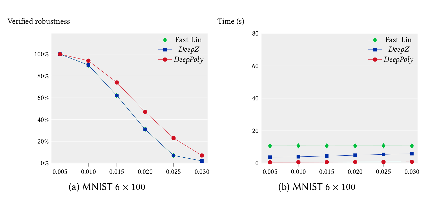
We ran our experiments for the feedforward networks on a 3.3 GHz 10 core Intel i9-7900X Skylake CPU with a main memory of 64 GB whereas our experiments for the convolutional networks were run on a 2.6 GHz 14 core Intel Xeon CPU E5-2690 with 512 GB of main memory. We first compare the precision and performance of DeepZ and DeepPoly vs Fast-Lin on the MNIST 6x100 network in single threaded mode. It can be seen that DeepZ has the same precision as Fast-Lin whereas DeepPoly is more precise while also being faster.
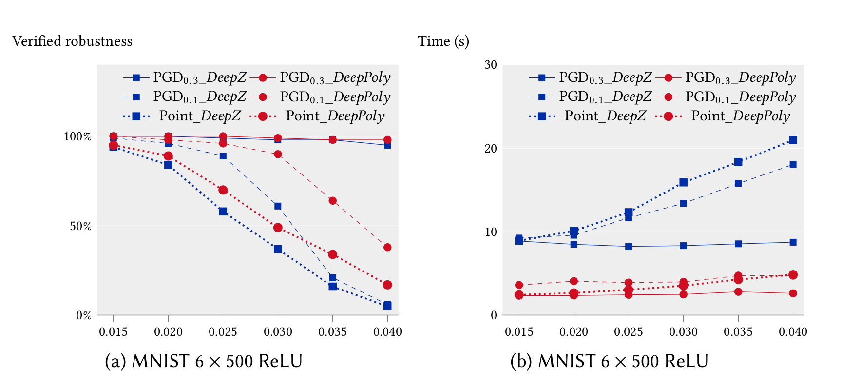
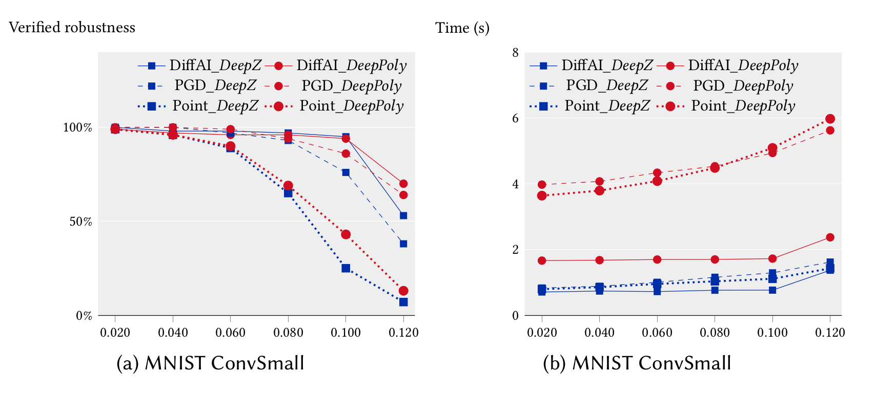
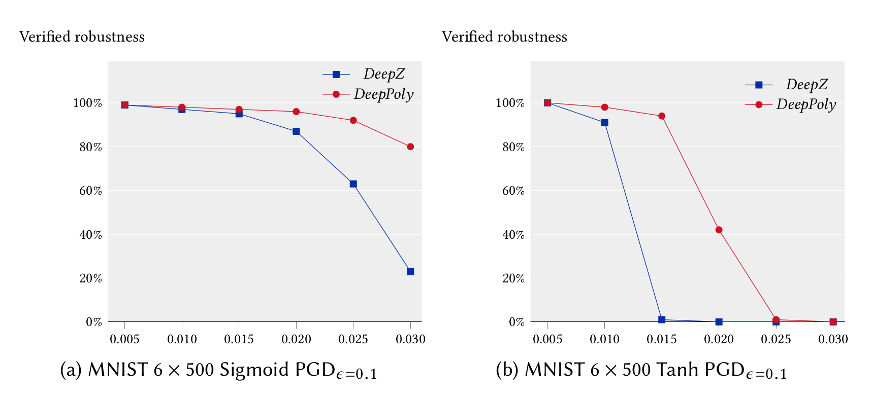
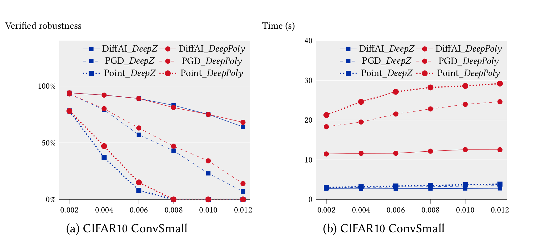
In the following, we compare the precision and performance of DeepZ and DeepPoly on a subset of the neural networks listed above in multi-threaded mode. In can be seen that DeepPoly is overall more precise than DeepZ but it is slower than DeepZ on the convolutional networks.
The table below compares the performance and precision of DeepZ and DeepPoly on our large networks trained with DiffAI.
<table aligh="center"> <tr> <td>Dataset</td> <td>Model</td> <td>ε</td> <td colspan="2">% Verified Robustness</td> <td colspan="2">% Average Runtime (s)</td> </tr> <tr> <td> </td> <td> </td> <td> </td> <td> DeepZ </td> <td> DeepPoly </td> <td> DeepZ </td> <td> DeepPoly </td> </tr> <tr> <td> MNIST</td> <td> ConvBig</td> <td> 0.1</td> <td> 97 </td> <td> 97 </td> <td> 5 </td> <td> 50 </td> </tr> <tr> <td> </td> <td> ConvBig</td> <td> 0.2</td> <td> 79 </td> <td> 78 </td> <td> 7 </td> <td> 61 </td> </tr> <tr> <td> </td> <td> ConvBig</td> <td> 0.3</td> <td> 37 </td> <td> 43 </td> <td> 17 </td> <td> 88 </td> </tr> <tr> <td> </td> <td> ConvSuper</td> <td> 0.1</td> <td> 97 </td> <td> 97 </td> <td> 133 </td> <td> 400 </td> </tr> <tr> <td> </td> <td> Skip</td> <td> 0.1</td> <td> 95 </td> <td> N/A </td> <td> 29 </td> <td> N/A </td> </tr> <tr> <td> CIFAR10</td> <td> ConvBig</td> <td> 0.006</td> <td> 50 </td> <td> 52 </td> <td> 39 </td> <td> 322 </td> </tr> <tr> <td> </td> <td> ConvBig</td> <td> 0.008</td> <td> 33 </td> <td> 40 </td> <td> 46 </td> <td> 331 </td> </tr> </table>The table below compares the timings of complete verification with ERAN for all ACASXu benchmarks.
<table aligh="center"> <tr> <td>Property</td> <td>Networks</td> <td colspan="1">% Average Runtime (s)</td> </tr> <tr> <td> 1</td> <td> all 45</td> <td> 15.5 </td> </tr> <tr> <td> 2</td> <td> all 45</td> <td> 11.4 </td> </tr> <tr> <td> 3</td> <td> all 45</td> <td> 1.9 </td> </tr> <tr> <td> 4</td> <td> all 45</td> <td> 1.1 </td> </tr> <tr> <td> 5</td> <td> 1_1</td> <td> 26 </td> </tr> <tr> <td> 6</td> <td> 1_1</td> <td> 10 </td> </tr> <tr> <td> 7</td> <td> 1_9</td> <td> 83 </td> </tr> <tr> <td> 8</td> <td> 2_9</td> <td> 111 </td> </tr> <tr> <td> 9</td> <td> 3_3</td> <td> 9 </td> </tr> <tr> <td> 10</td> <td> 4_5</td> <td> 2.1 </td> </tr> </table> <table>The table below shows the certification performance of PRIMA (refinepoly with Precise Multi-Neuron Relacations). For MLPs we use CPU only certificaiton, while we use GPUPoly for the certification of the convolutional networks.
<thead> <tr> <th>Network</th> <th>Data subset</th> <th>Accuracy</th> <th>Epsilon</th> <th>Upper Bound</th> <th>PRIMA certified</th> <th>PRIMA runtime [s]</th> <th>N</th> <th>K</th> <th>Refinement</th> <th>Partial MILP (layers/max_neurons)</th> </tr> </thead> <tbody> <tr> <td>MNIST</td> <td></td> <td></td> <td></td> <td></td> <td></td> <td></td> <td></td> <td></td> <td></td> <td></td> </tr> <tr> <td>6x100 [NOR]</td> <td>first 1000</td> <td>960</td> <td>0.026</td> <td>842</td> <td>510</td> <td>159.2</td> <td>100</td> <td>3</td> <td>y</td> <td></td> </tr> <tr> <td>9x100 [NOR]</td> <td>first 1000</td> <td>947</td> <td>0.026</td> <td>820</td> <td>428</td> <td>300.63</td> <td>100</td> <td>3</td> <td>y</td> <td></td> </tr> <tr> <td>6x200 [NOR]</td> <td>first 1000</td> <td>972</td> <td>0.015</td> <td>901</td> <td>690</td> <td>223.6</td> <td>50</td> <td>3</td> <td>y</td> <td></td> </tr> <tr> <td>9x200 [NOR]</td> <td>first 1000</td> <td>950</td> <td>0.015</td> <td>911</td> <td>624</td> <td>394.6</td> <td>50</td> <td>3</td> <td>y</td> <td></td> </tr> <tr> <td>ConvSmall [NOR]</td> <td>first 1000</td> <td>980</td> <td>0.12</td> <td>746</td> <td>598</td> <td>41.7</td> <td>100</td> <td>3</td> <td>n</td> <td>1/30</td> </tr> <tr> <td>ConvBig [DiffAI]</td> <td>first 1000</td> <td>929</td> <td>0.3</td> <td>804</td> <td>775</td> <td>15.3</td> <td>100</td> <td>3</td> <td>n</td> <td>2/30</td> </tr> <tr> <td>CIFAR-10</td> <td></td> <td></td> <td></td> <td></td> <td></td> <td></td> <td></td> <td></td> <td></td> <td></td> </tr> <tr> <td>ConvSmall [PGD]</td> <td>first 1000</td> <td>630</td> <td>2/255</td> <td>482</td> <td>446</td> <td>13.25</td> <td>100</td> <td>3</td> <td>n</td> <td>1/100</td> </tr> <tr> <td>ConvBig [PGD]</td> <td>first 1000</td> <td>631</td> <td>2/255</td> <td>613</td> <td>483</td> <td>175.9</td> <td>100</td> <td>3</td> <td>n</td> <td>2/512</td> </tr> <tr> <td>ResNet [Wong]</td> <td>first 1000</td> <td>289</td> <td>8/255</td> <td>253</td> <td>249</td> <td>63.5</td> <td>50</td> <td>3</td> <td>n</td> <td></td> </tr> <tr> <td>CNN-A [MIX]</td> <td>Beta-CROWN 100</td> <td>100</td> <td>2/255</td> <td>69</td> <td>50</td> <td>20.96</td> <td>100</td> <td>3</td> <td>n</td> <td>1/100</td> </tr> <tr> <td>CNN-B [ADV]</td> <td>Beta-CROWN 100</td> <td>100</td> <td>2/255</td> <td>83</td> <td>43</td> <td>259.7</td> <td>100</td> <td>3</td> <td>n</td> <td>1/250</td> </tr> </tbody> </table>More experimental results can be found in our papers.
Contributors
-
Mark Niklas Müller (lead contact) - mark.mueller@inf.ethz.ch
-
Gagandeep Singh (contact for ELINA) - ggnds@illinois.edu gagandeepsi@vmware.com
-
Mislav Balunovic (contact for geometric certification) - mislav.balunovic@inf.ethz.ch
-
Gleb Makarchuk (contact for FConv library) - hlebm@ethz.ch gleb.makarchuk@gmail.com
-
Anian Ruoss (contact for spatial certification) - anruoss@ethz.ch
-
François Serre (contact for GPUPoly) - serref@inf.ethz.ch
-
Adrian Hoffmann - adriahof@student.ethz.ch
-
Jonathan Maurer - maurerjo@student.ethz.ch
-
Christoph Müller - christoph.mueller@inf.ethz.ch
License and Copyright
- Copyright (c) 2020 Secure, Reliable, and Intelligent Systems Lab (SRI), Department of Computer Science ETH Zurich
- Licensed under the Apache License