Awesome

Flood-Mapping-Using-Satellite-Images

MSc Thesis - Data Science - UoP & NCSR "Demokritos"

<h2> Download The Dataset </h2>

<b>First Option:</b><br> Visit the following link: <br> https://mlhub.earth/data/c2smsfloods_v1 (you need to create an account first)
<b>Second Option:</b><br> The dataset is available for access through Google Cloud Storage bucket at: gs://senfloods11/

You can access the dataset bucket using the gsutil command line tool. If you would like to download the entire dataset (~14 GB) you can use gsutil rsync to clone the bucket to a local directory. The -m flag is recommended to speed downloads. The -r flag will download sub-directories and folder recursively. See the example below.

<i> $ gsutil -m rsync -r gs://sen1floods11 /YOUR/LOCAL/DIRECTORY/HERE </i>

<h2> Dataset Information </h2>

The dataset used is named as <b>Sen1Floods11</b> and it is comprised with Sentinel 1 & 2 images with the corresponding ground truth masks. The dataset contains two main folders (<b>flood_events & perm_water</b>) as shown below:

In this study we are only using the images included on the <b>Flood Events</b> folder and eliminate the permanent water images. The <b>flood_events</b> folder is further splitted into 2 subfolders as shown in the image below:

The <b> HandLabeled </b> subfolder is splitted into 5 subfolders from which we are not using the "JRCWaterHand".

While the <b>WeaklyLabeled</b> folder is splitted into 3 from which we are not using the "S2IndexLabelWeak".

<h2> Flood Events </h2> <h3> Hand Labeled </h3> <p center="left"> This subfolder contains one folder <b> S1Hand</b> which consists of sentinel 1 image patches with two polarization bands (VH & VV) and another one called <b> S2Hand </b> which includes Sentinel 2 image patches with all <b>13 spectral bands</b>. It should be noticed that not all bands share the same spatial resolution, thus if needed an extra processing (pansharpening) should be applied. The size of the patches is 512x512 within the coordinate system EPSG:4326 - WGS 84 - Geographic. The rest folders are the coresponding ground trouth mask, each one being created with a different method. The areas of study are parts of 12 countries as shown below: </p> <p float="left"> <img src="./imgs/HandLabeledTable.png" width="500" /> </p> <h3> Weakly Labeled </h3> <p float="left"> <img src="./imgs/WeaklyLabeledTable.png" width="500" /> </p> As can be seen the size of the Weakly labeled dataset is much larger than the hand labeled one. It should be noted that weakly labeled patches are not overlapping with the hand labeled patches, but they are geographically close. <h2> Clean the Dataset - Pre Process </h2> <h3> Hand Labeled </h3> <p center="left"> After visually checking the dataset with manually loading image patches on a free and open Geographic Information System software called QGIS, we noticed that many images contain corroded pixels with no information or the number with flooded pixels is significant lower than the background pixels. Additionally it was noticed that a large number of sentinel 2 images are heavily or totally covered with clouds. Bellow is an illustration of a sentinel 2 image tile blocked with clouds, the corresponding sentinel 1 tile and the respective ground truth. The initial image tiles of 512x512 size were splited into patches of 128x128, so from each itinial image 16 patches were created. The splitting process in a google colab environment took 8 to 10 hours to complete.</p> <p center="left"> Another critical issue was the imbalance between the number of flooded pixels and the background pixels. In order to overcome all these challenges and create a coherent multimodal dataset, we eliminated patches completely covered with clouds, with no flooded pixels or corroded pixels but also the patches with unbalanced number of flooded pixels and background pixels. The remaining number of patches per geographic area is illustrated in Table 4.1. with a total number of images of 577.</p> <p float="left"> <img src="./imgs/s2.png" width="200" /> <img src="./imgs/s1.png" width="200" /> <img src="./imgs/label.png" width="200" /> </p> <p float="left"> <img src="./imgs/S2_half.png" width="200" /> <img src="./imgs/Label_half.png" width="200" /> </p> <h3> Weakly Labeled </h3> <p center="left"> The initial total number of images were 4384. Each image was splitted into 16 patches of a size 128x128 pixels, resulting in 70144 patches in total. From these we remove the patches having at least one cropped pixel labeled as (-1), patches were the number of flooded pixels were more than 50% than the background pixels and patches with with background pixels more than 50% of the flooded pixels, resulting in a dataset comprised of 6835 patches. Since the number of patches were still very high and not easy to handle, only the first 50 patches from each geographic area we kept, resulting in 600 patches in total. </p>

The link for the new dataset: https://uopel-my.sharepoint.com/:f:/g/personal/dit2025dsc_office365_uop_gr/EjZZUSHVyv1LozsRfnTt7uEBKoDEbOsyDsCOzMPi0X02lQ?e=gBMJub

<h2> Experiments </h2> <p center="left">Experiments were splited into three parts, with each one based on a different semantic segmentation scheme. The first one is based on a Fully Convolutional Neural Network called U-NET, the second approach is based on a Random Forest and a set of hand crafted features while the last one is based on the concept of Transfer Learning using as a backbone the VGG16 model.</p> <h3>1. U-NET </h3> <p center="left">U-Net is a convolutional neural network that was developed for biomedical image segmentation. The network is based on the <b>fully convolutional network</b> and its architecture was modified and extended to work with fewer training images and to yield more precise segmentations. The network consists of a contracting path (convolution) and an expansive path (deconvolution), which gives it the u-shaped architecture. The contracting path is a typical convolutional network that consists of repeated application of convolutions, each followed by a rectified linear unit (ReLU) and a max pooling operation. During the contraction, the spatial information is reduced while feature information is increased. The expansive pathway combines the feature and spatial information through a sequence of up-convolutions and concatenations with high-resolution features from the contracting path. [https://en.wikipedia.org/wiki/U-Net#cite_note-Shelhamer_2017-2] </p>

Single-Modal - UNET

Hand Labeled
Source & Labels	IOU	Acc
S1Hand & S1OtsuLabelHand	0.89	0.94
S2Hand & LabelHand	0.47	0.72

Weakly Labeled
Source & Labels	IOU	Acc
S1Hand & S1OtsuLabelWeak	0.81	0.87

Weakly Supervised
Trained On	Tested on	IOU	Acc
S1Hand & S1OtsuLabelWeak	S1OtsuLabelHand	0.77	0.86

Multi-Modal - UNET

Hand Labeled
Source & Labels	IOU	Acc
S1Hand - S2Hand & S1OtsuLabelHand	0.72	0.82
S1Hand - S2Hand & LabelHand	0.42	0.71

<h3> 2. Random Forest - Feature Engineering </h3> Feature based segmentation using Random Forest <p center="left">For this set of experiments a various hand crafted features were utilized from both sentinel 1 and sentinel 2 raw spectral bands. More specifically from optical bands were constructed the NDVI and NDWI while from sentinel 1 the devision between VV and VH. Apart from these futures three more kernel based features were con- structed based on VH and NIR bands respectively. Those are the median filter with and variance filters with kernel size of 3 and the roberts edge detection filter.</p>

Single-Modal - RF

Hand Labeled
Source & Labels	IOU	Acc
S1Hand & S1OtsuLabelHand	0.79	0.89
S2Hand & LabelHand	0.87	0.93

Weakly Labeled
Source & Labels	IOU	Acc
S1Weak & S1OtsuLabelWeak	0.81	0.90

Weakly Supervised
Trained On	Tested on	IOU	Acc
S1Weak & S1OtsuLabelWeak	S1Hand + S1OtsuLabelHand	0.77	0.88

Multi-Modal - RF

Hand Labeled
Source & Labels	IOU	Acc
S1Hand - S2Hand & S1OtsuLabelHand	0.84	0.92
S1Hand - S2Hand & LabelHand	0.87	0.93

<h3> 3. Transfer Learning - VGG16 </h3>  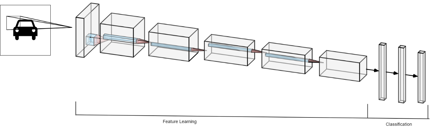<p center="left">In the current study the VGG16 architecture pretrained on the Imagenet pub- licly available data is being used, while the Sen1Floods11 dataset is used for fine tuning. Lastly, the classification part is handled by a random forest. </p>

Single-Modal - Transfer Learning (R NIR SWIR, VV+VH +VH/VV)

Hand Labeled
Source & Labels	IOU	Acc
S1Hand & S1OtsuLabelHand	0.84	0.92
S2Hand & LabelHand	0.47	0.65

Weakly Labeled
Source & Labels	IOU	Acc
S1Hand & S1OtsuLabelWeak	0.86	0.92

Weakly Supervised
Trained On	Tested on	IOU	Acc
S1Hand & S1OtsuLabelWeak	S1Hand + S1OtsuLabelHand	0.83	0.91

Multi-Modal - Transfer Learning (VH+RED+NIR)

Hand Labeled
Source & Labels	IOU	Acc
S1Hand - S2Hand & S1OtsuLabelHand	0.73	0.85
S1Hand - S2Hand & LabelHand	0.55	0.71

<h2> Credits </h2> Credits to <a href="https://github.com/bnsreenu">Dr. Sreenivas Bhattiprolu</a> for his excellent python and machine learning tutorials which I used through out my thesis.