Awesome

Please check here for complete documentation

Example

The below data science flavored code is a well-known iris example from scikit-learn.

"""
Example of Logistic regression using scikit-learn
https://scikit-learn.org/stable/auto_examples/linear_model/plot_iris_logistic.html
"""

import matplotlib.pyplot as plt
import numpy as np
from sklearn import datasets
from sklearn.inspection import DecisionBoundaryDisplay
from sklearn.linear_model import LogisticRegression


def load_data():
    # import some data to play with
    iris = datasets.load_iris()
    X = iris.data[:, :2]  # we only take the first two features.
    Y = iris.target

    return X, Y


def model_fit(X: np.ndarray, Y: np.ndarray, C: float = 1e5):
    logreg = LogisticRegression(C=C)
    logreg.fit(X, Y)

    return logreg


def generate_plots(X: np.ndarray, Y: np.ndarray, logreg: LogisticRegression):
    _, ax = plt.subplots(figsize=(4, 3))
    DecisionBoundaryDisplay.from_estimator(
        logreg,
        X,
        cmap=plt.cm.Paired,
        ax=ax,
        response_method="predict",
        plot_method="pcolormesh",
        shading="auto",
        xlabel="Sepal length",
        ylabel="Sepal width",
        eps=0.5,
    )

    # Plot also the training points
    plt.scatter(X[:, 0], X[:, 1], c=Y, edgecolors="k", cmap=plt.cm.Paired)

    plt.xticks(())
    plt.yticks(())

    plt.savefig("iris_logistic.png")

    # TODO: What is the right value?
    return 0.6


## Without any orchestration
def main():
    X, Y = load_data()
    logreg = model_fit(X, Y, C=1.0)
    generate_plots(X, Y, logreg)


## With runnable orchestration
def runnable_pipeline():
    # The below code can be anywhere
    from runnable import Catalog, Pipeline, PythonTask, metric, pickled

    # X, Y = load_data()
    load_data_task = PythonTask(
        function=load_data,
        name="load_data",
        returns=[pickled("X"), pickled("Y")],  # (1)
    )

    # logreg = model_fit(X, Y, C=1.0)
    model_fit_task = PythonTask(
        function=model_fit,
        name="model_fit",
        returns=[pickled("logreg")],
    )

    # generate_plots(X, Y, logreg)
    generate_plots_task = PythonTask(
        function=generate_plots,
        name="generate_plots",
        terminate_with_success=True,
        catalog=Catalog(put=["iris_logistic.png"]),  # (2)
        returns=[metric("score")],
    )

    pipeline = Pipeline(
        steps=[load_data_task, model_fit_task, generate_plots_task],
    )  # (4)

    pipeline.execute()

    return pipeline


if __name__ == "__main__":
    # main()
    runnable_pipeline()

1. Return two serialized objects X and Y.
2. Store the file iris_logistic.png for future reference.
3. Define the sequence of tasks.
4. Define a pipeline with the tasks

The difference between native driver and runnable orchestration:

!!! tip inline end "Notebooks and Shell scripts"

You can execute notebooks and shell scripts too!!

They can be written just as you would want them, *plain old notebooks and scripts*.

- X, Y = load_data()
+load_data_task = PythonTask(
+    function=load_data,
+     name="load_data",
+     returns=[pickled("X"), pickled("Y")], (1)
+    )

-logreg = model_fit(X, Y, C=1.0)
+model_fit_task = PythonTask(
+   function=model_fit,
+   name="model_fit",
+   returns=[pickled("logreg")],
+   )

-generate_plots(X, Y, logreg)
+generate_plots_task = PythonTask(
+   function=generate_plots,
+   name="generate_plots",
+   terminate_with_success=True,
+   catalog=Catalog(put=["iris_logistic.png"]), (2)
+   )


+pipeline = Pipeline(
+   steps=[load_data_task, model_fit_task, generate_plots_task], (3)

• Domain code remains completely independent of driver code.
• The driver function has an equivalent and intuitive runnable expression
• Reproducible by default, runnable stores metadata about code/data/config for every execution.
• The pipeline is runnable in any environment.

Documentation

More details about the project and how to use it available here.

Installation

The minimum python version that runnable supports is 3.8

pip install runnable

Please look at the installation guide for more information.

Pipelines can be:

Linear

A simple linear pipeline with tasks either python functions, notebooks, or shell scripts

Parallel branches

Execute branches in parallel

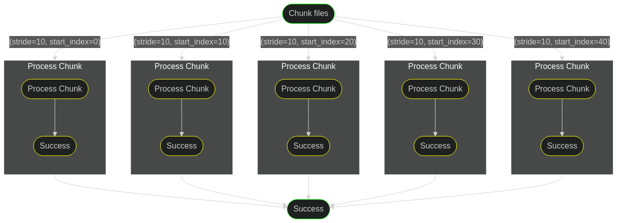
loops or map

Execute a pipeline over an iterable parameter.

Arbitrary nesting

Any nesting of parallel within map and so on.